Download PDF
Use this page to insert new HTML entries, then delete them from the page itself so as not to clutter it
Complete archive of all research reports and briefs
Download PDF
Download PDF
MARRIAGE DESERTS
Mapping America’s Family Divide
Chris Bullivant, Ken Burchfiel
April 2026
DRAFT 1
CONTENTS PAGE
We are indebted to several colleagues for their assistance in developing these maps. John Iceland of Penn State provided an external review of the methodology and results. Brad Wilcox offered valuable guidance on the scope of the report and the distinction between marriage deserts (share of adults married) and married-family deserts (share of households with children headed by married couples). Lyman Stone gave critical feedback on the use of the 2020 decennial Census, including the recommendation to group tract-level data by PUMA for more reliable calculations, and served as a key internal check throughout the project. Wendy Wang provided generous input during drafting to ensure the analysis met IFS research standards and supported the development of this map-based approach. Grant Bailey advised on suitable data sources and its presentation. Alysse ElHage provided invaluable editorial support throughout. We are also grateful to the team at Bevy Commerce, particularly Jafar Mahmood, for technical and design support in embedding the maps on the IFS website.
An author (Chris Bullivant) used AI-based tools in early drafts for proofreading and terminology consistency; all analysis and conclusions are the author’s own.
Include Top 10 Marriage Deserts, Top 10 Married-Family Deserts
[Complete closer to final draft].
This report accompanies two maps of the United States that are available online at the Institute for Family Studies website (ifstudies.org/marriagedeserts). These maps allow the user to view marriage and married-family shares within any part of the United States. The data informing these maps is made available at the same location in a series of tables ranking areas by their marriage rates and share of married families. The maps and the tables are both based on data from the 2020 US Census.
In this report we draw from these tables to present the Top 10 Marriage Deserts and Top 10 Married-Family Deserts in the United States. These areas are where marriage rates are low, and where the share of households with children headed by married couples is low.
We also list the Top 10 Marriage Gardens and Top 10 Married-Family Gardens. These are areas where the marriage rate is high, and where the share of households with children headed by married couples is high.
The areas we use to measure are Public Use Microdata Areas (PUMAs), roughly comparable units with an average size of 135,000 people. After presenting the Top 10 individual-PUMA deserts and gardens, we will then show top-10 lists of grouped PUMAs that share the same marriage or married-family category.
The assets described in this report are:
|
INDIVIDUAL PUMAs |
|
GROUPED PUMAs |
|
Marriage Maps and Tables |
|
Marriage Maps and Tables |
|
1: Map of PUMAs by marriage category 2: Table of PUMAs by marriage category 3: Table of top marriage deserts 4: Table of top marriage gardens |
|
9: Map of grouped marriage deserts and gardens 10: Table of top grouped marriage deserts 11: Table of top grouped marriage gardens |
|
Married-Family Maps and Tables |
|
Married-Family Maps and Tables |
|
5: Map of PUMAs by married-family category 6: Table of PUMAs by married-family category 7: Table of top married-family deserts 8: Table of top married-family gardens |
|
12: Map of grouped married-family deserts and gardens 13: Table of top grouped married-family deserts 14: Table of top grouped married-family gardens |
Marriage Desert: A PUMA where the share of householders aged 15-64 who are married is below 33%. (Here we look simply at the share of adults who are married versus not married—the latter which could include single, never-married, divorced, or widowed people. Those areas with very low levels of marriage are specifically termed marriage deserts.)
Marriage Garden: A PUMA where the share of householders aged 15-64 who are married is at or above 61%.
Married-Family Desert: A PUMA in which fewer than 52% of households with children are headed by a married couple. (In this report, 'children' refers to what the Census defines as 'own children' (rather than 'related children'); see methodology section for more details.
Married-Family Garden: A PUMA in which the share of households with children headed by a married couple is at or above 79%.
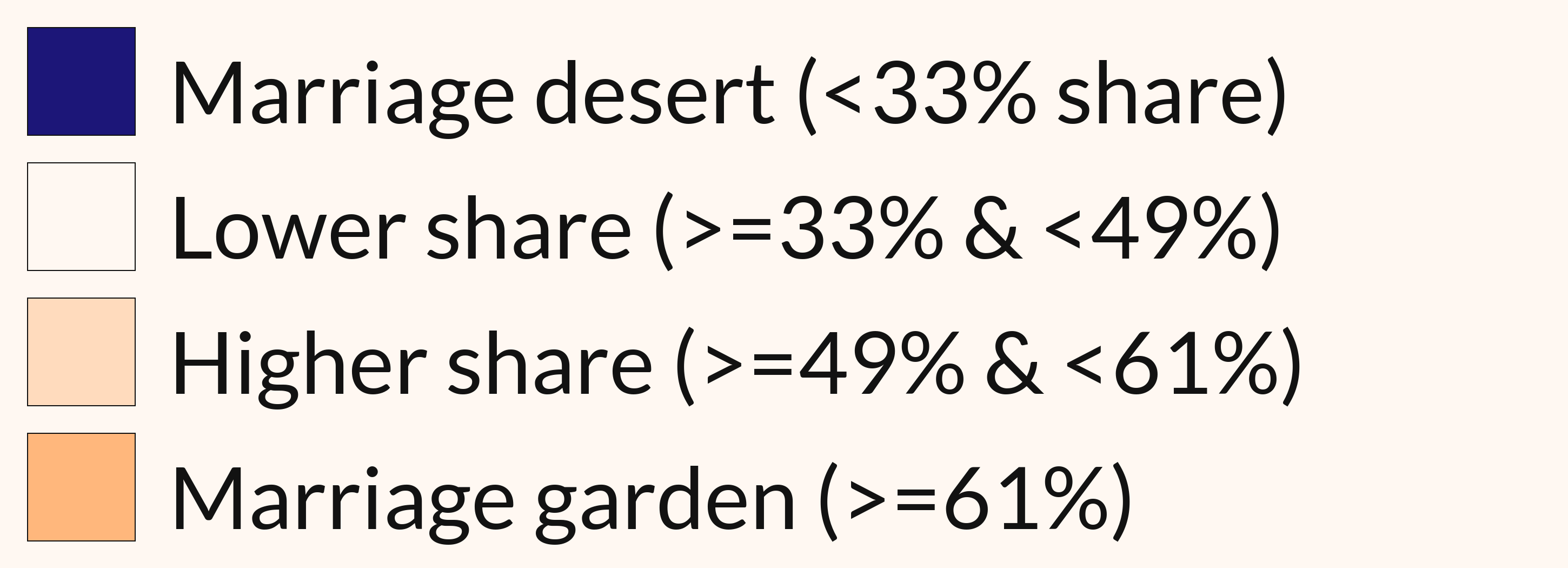
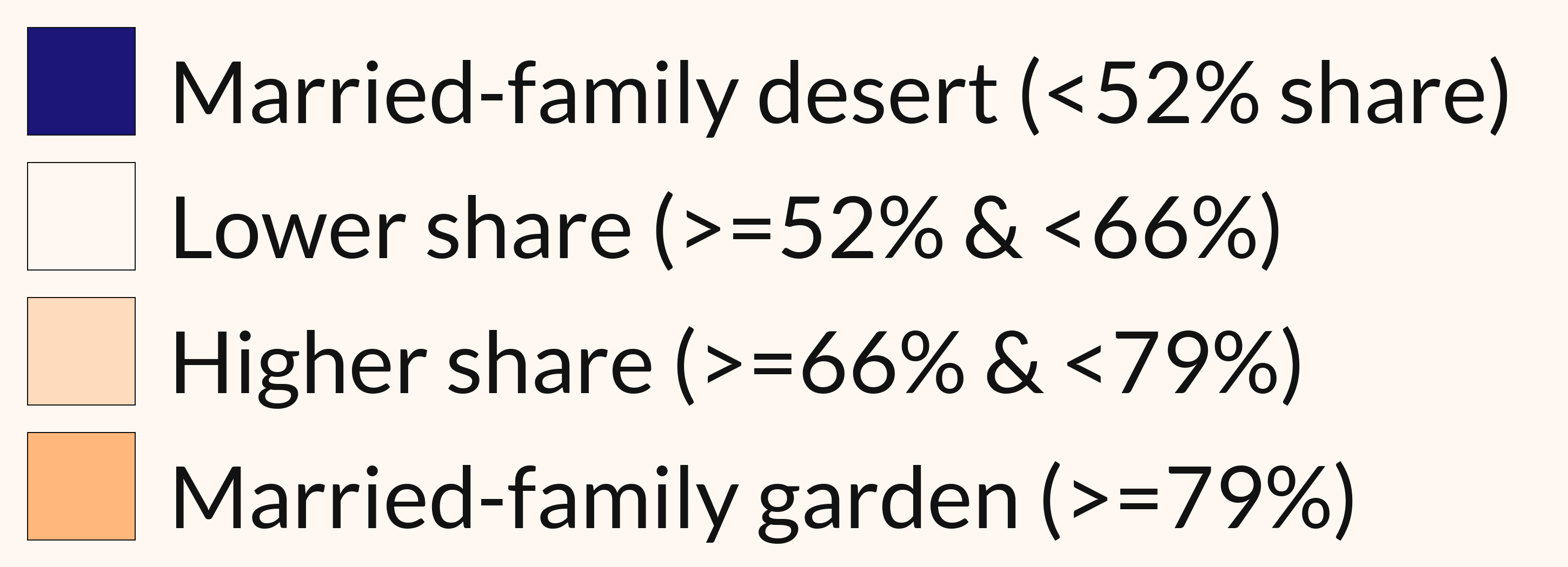
The categorical legend used for marriage and married-family maps are as follows.
Further details on how and why we established these categories are available in the methodology section.
Marriage categories
Married-family categories
Why this report?
Neighborhood family structures—whether experienced in tenements, apartments, public schools, or the local store—inform each other with a complex set of norms. As shown in research by Harvard economist Raj Chetty, “the most predictive factor of upward mobility in a community was the share of homes with two parents present in the household.”i
And yet, there is a sharp divide in the experience of family across the United States dependent upon income. As IFS Senior Fellow Brad Wilcox and report author Chris Bullivant wrote in a previous paper,ii higher levels of marriage and stability were prevalent among high-income families. Conversely, lower levels of marriage and stability were prevalent among low-income families.
This “social capital divide” is of concern because, across multiple metrics, children growing up in stable-married families have better life outcomes than their counterparts who grow up in less-stable cohabiting or single-parent households.
So that the predictive, though not deterministic, quality of the share of homes with two parents present in the household begs the question: where are these neighborhoods? And where aren’t they?iii Because perhaps, if we can see where they are, it may be easier to bridge the social-capital divide to create equal access to stable, married family life and the relational security it confers.
Marriage deserts
This work was inspired by the Opportunity Atlas published by Opportunity Insights--in particular, their upward mobility maps, which include the share of people who are married by age 30.iv Their maps reveal a patchwork quality to marriage rates at a census tract level. Bullivant described the low marriage rates neighborhoods in these maps as “marriage deserts” in an article with Brad Wilcox.v Just as it is harder to buy healthier groceries in a “food desert,” it is likely harder to enter into stable married families in a “marriage desert.” This is simply where relationships styles are learned in the context of existing relationships.
Inspired by the Opportunity Insights maps, we wanted to create our own, humbler family-focused versions that homed in on two measures:
The share of householders aged 15-64 who are married.
A sense of the share of households with children that are stable, two-parent homes. (In this case, we use married couples as a proxy.)
What this report does not do
Beyond listing and describing the Top 10 marriage deserts/gardens, and married-family deserts/gardens, we offer minimal analysis as to causes.
It is also beyond the scope of our research to establish a causal relationship between low rates of marriage and low rates of married families, or their converse, high rates of marriage and high rates of married families. While the connection may seem obvious, there are areas where higher rates of marriage do not correlate with higher rates of married families, and there are areas where low marriage rates correlate with higher shares of married families.
However, these maps are presented with the knowledge that areas of low marriage and weak family stability are more prone to less upward social mobility. And we hope that these are a useful tool for inspiring further research and analysis.
The full table and map visualizing the share of householders aged 15-64 who are married are available here. The Top 10 marriage desert and top 10 marriage gardens are pulled from these assets.
Map:
Table:
These are the top ten marriage deserts in the United States.
In this report, marriage deserts are defined as Public Use Microdata Areas (PUMAs) in which the share of householders aged 15 to 64 who are married falls below 33 percent (the rounded 10th percentile for this metric), representing the lowest-observed marriage rates nationally.
The table below ranks the ten PUMAs with the lowest shares of married householders ages 15–64. Across these areas, the married share of householders ranges from 13.0 percent to 16.9 percent. This implies that more than 80 percent of householders ages 15–64 in these PUMAs are not married.
These marriage deserts are located in ten major U.S. metropolitan areas across seven states—Georgia, Illinois, Massachusetts, Michigan, Missouri, Ohio, and Wisconsin—as well as the District of Columbia. Ohio appears three times in the top ten, making it the only state represented more than once. All ten PUMAs are located east of the Rocky Mountains. (Original PUMA names were simplified for easier readability.)
These are the ten largest marriage gardens in the United States.
In this report, marriage gardens are defined as Public Use Microdata Areas (PUMAs) in which the share of householders aged 15 to 64 who are married is at least 61%, representing the highest-observed marriage shares nationally.
The table below ranks the ten PUMAs with the highest shares of married householders aged 15–64. Across these areas, the married share of householders ranges from 73.9 percent to 78.6 percent. This implies that around three in four householders aged 15–64 in these PUMAs are married, roughly the inverse of the pattern observed in the nation’s largest marriage deserts.
These marriage gardens are located in ten counties or county-equivalent areas across six states—Connecticut, Florida, New Jersey, Tennessee, Texas, and Utah. Texas appears three times in the top ten, while Utah and New Jersey each appear twice. Notably, none of the top-10 marriage gardens are located in major U.S. cities.
The differences between the Top 10 Marriage Deserts and the Top 10 Marriage Gardens are stark, with a 60+ percentage-point spread between these two extremes:
Marriage deserts: 13.0%–16.9% married
Marriage gardens: 73.9%–78.6% married
Even the marriage desert in tenth place, in Chicago, 16.9%, has less than one quarter the marriage share of the 10th-ranked marriage garden in Thompson Station Town/Fairview, 73.9%. This does not appear to describe small variations around shared national norms, but rather two distinct family-formation regimes, so stark it could even be described as family structure polarization.
No state appears on both top ten lists, suggesting an element of geographic polarization in family structure at the extremes. At the same time, this comparison should not be overinterpreted: a broader review of national maps shows that it is common for states to contain both marriage deserts and marriage gardens, often in close geographic proximity. The polarization observed here reflects the most extreme cases, not complete state-level segregation.
Ohio stands out as a negative outlier. Three Ohio PUMAs—Cleveland, Columbus, and Cincinnati—appear among the top ten marriage deserts, while none appear among the top ten marriage gardens. In the full national distribution, Ohio contains seven marriage gardens, with the largest—Delaware County (South), Ohio—ranking 41st nationally. Further research examining changes in marriage shares over time may help clarify whether Ohio’s pattern reflects long-term post-industrial family decline distinct from the experiences of coastal, urbanized areas. Ohio stands in contrast to Texas, which features three marriage gardens in the top 10 while not appearing in our list of the top 10 marriage deserts.
What do these patterns imply for children? While the analysis above focuses on the share of householders aged 15–64 who are married, the underlying motivation is to understand how local family structure shapes the social capital environments in which children are raised. A substantial body of research indicates that children’s life outcomes are strongly influenced by relational stability within the family of origin, as well as by the prevalence of married-couple households in their surrounding community.
The top ten married-family deserts and top ten married-family gardens are therefore identified using the share of households with children of their own that are headed by married couples. This is with a view to considering a child’s relational security—the degree of stability, continuity, and reliability in the family and community relationships that surround them.
The Top 10 married-family deserts and top 10 married-family gardens are pulled from these assets.
Map:
Table:
In this analysis, married-family deserts are defined as Public Use Microdata Areas (PUMAs) in which the share of households with children that are headed by a married couple falls below 52 percent. In these areas, children are less likely to be raised in a household headed by married parents and less likely to be surrounded by peers growing up in married-couple families—conditions associated with lower levels of relational security at both the household and neighborhood level.
The table below ranks the ten PUMAs with the lowest shares of households with children headed by a married couple. Across these areas, the share of households with children headed by a married couple ranges from 18.0 percent to 25.7 percent. In all ten of these married-family deserts, fewer than one in four households with children are headed by a married couple.
Put differently, in these PUMAs, children are three to four times more likely to live in households with children that are not headed by married parents than in households that are.
These ten married-family deserts are located in eight major U.S. metropolitan areas across seven states—Georgia, Illinois, Kentucky, Michigan, Missouri, Ohio, and Wisconsin—and the District of Columbia. Chicago and Detroit each contain two married -family deserts. As with the marriage deserts, all ten married -family deserts are located east of the Rocky Mountains.
In this analysis, married-family gardens are defined as Public Use Microdata Areas (PUMAs) in which the share of households with children that are headed by a married couple is at least 79 percent. In these areas, children are most likely to be raised in households headed by married parents and to be surrounded by peers growing up in married-couple families—conditions associated with higher levels of relational security at both the household and neighborhood level.
The table below ranks the ten PUMAs with the highest shares of households with children headed by a married couple, among PUMAs with substantial numbers of households with children. Across these areas, the share of households with children headed by a married couple ranges from 86.7 percent to 88.9 percent. In all ten married-family gardens, fewer than one in seven households with children are not headed by a married couple.
Put differently, in these PUMAs, children are six to eight times more likely to live in households with children headed by married parents than in households with children that are not headed by married parents.
These ten married-family gardens are located primarily in the suburban and exurban communities of major U.S. metropolitan areas across seven states—California, Connecticut, Illinois, Massachusetts, New Jersey, Texas, and Utah. California, New Jersey, and Utah each contain two married-family gardens in the top ten.
The differences between the Top 10 Married-Family Deserts and the Top 10 Married-Family Gardens are stark, with a difference of roughly 70 percentage points between the extremes.
Lowest married-family desert: 18% of households with kids headed by a married couple
Highest married-family garden: 89% of households with kids headed by a married couple
Married-couple households constitute a supermajority of families with children in the top 10 married-family gardens (>86%), but only a small minority in the top 10 married-family deserts (<26%). The household composition of the top married-family deserts is effectively the inverse of that found in the top married-family gardens.
As with the marriage deserts/gardens, this comparison between married-family deserts and gardens demonstrates not just a variance around shared national norms, but a structural divergence in family structures. Over the course of childhood, these differences imply substantially different levels of exposure to married-couple households in children’s everyday social environments.
In the top 10 married-family deserts, children are three to four times more likely to live in households with children that are not headed by married parents.
In the top 10 married-family gardens, children are six to eight times more likely to live in households with children that are headed by married parents.
This will effect a significant discrepancy in lived experience for children growing up in these distinct environments. Those in married-family gardens grow up with married parents, in neighborhoods, schools, and after-school activities where most peers experience the same. These children will be observing marriage as a stable, ordinary feature of adult life. This will create stronger social capital networks, with a greater alignment between school, families, and community, overlapping stable inter-family interactions over a childhood and adolescence, creating denser networks of adult supervision, stable peer networks, and deep relational literacy.
For children in married-family deserts, by contrast, it is likely that there will be much greater churn in adult relationship stability, and greater inconsistency in supervision, where marriage and stable relationship bonds are atypical or distant from everyday norms—both for themselves and their peers. Greater intergenerational kinship, such as grandparent care, and demand on public resources such as schools may seek to compensate for this gap; however, it is likely that children in these married-family deserts will still experience less social capital, and diminished relational literacy, than those in to married-family gardens.
The top marriage gardens have twice the number of children as the top marriage deserts
The preceding analysis focuses on the share of households with children that are headed by married couples. An additional question is whether places with different family structures also differ in the overall prevalence of households with children. In other words, do married-family deserts and married-family gardens differ not only in how children are raised, but in how common it is for households to include children at all?
A clear pattern emerges when comparing the top ten married-family deserts with the top ten married-family gardens. PUMAs with markedly different family structures also differ substantially in the share of households that include children.
Among the top ten married-family deserts, the share of households with children ranges from a low of 14.9 percent in Detroit, Michigan, to a high of 26.4 percent in Chicago (West), Illinois. In contrast, among the top ten married-family gardens, the share of households with children ranges from 34.0 percent in Northfield and New Trier Townships, Illinois, to 57.5 percent in Utah County (West), Utah.
On average, households with children account for 21.0 percent of all households in the top ten married-family deserts, compared with 44.0 percent in the top ten married-family gardens. In practical terms, the share of households with children is approximately twice as high in the top married-family gardens as in the top married -family deserts.
This pattern is consistent with prior research showing that fertility in the United States is increasingly concentrated among married households and those with greater economic stability. Research by IFS Senior Fellow Lyman Stone, for example, finds that recent declines in fertility have been driven disproportionately by lower birth rates among the unmarriedvi and among lower-income populations.vii While the present analysis does not establish causality, the association between married-family structure and higher concentrations of households with children suggests that family norms and household formation are closely intertwined with contemporary fertility patterns.
Table: Top 10 Married-Family Gardens including percentage of households with children as a share of all households.
This comparison describes a considerable difference in local environments, especially as experienced by children.
Married-family deserts appear, on this evidence, to function increasingly as adult-oriented or post-family spaces, while married-family gardens appear to be environments that are more conducive to having and raising children. For children growing up in married-family deserts, this means not only being raised within a context of greater relational instability, but also living in environments where having children in the household is itself less common. Parenting, as well as marriage, is therefore less frequently observed as a dominant adult role within the community.
These differences have implications for schools, housing markets, tax bases, welfare systems, local politics, and the balance between services oriented toward children and those oriented toward older populations. Over time, environments with fewer children may also face challenges in sustaining the institutions and informal networks that support family life.
It is notable that within the top ten married-family deserts, even where the share of households with children headed by married couples is relatively higher, the overall share of households with children does not increase substantially. This pattern may point to deeper structural constraints on family formation in these neighborhoods. One possible interpretation is a process of social-capital erosion in which unstable relationship norms, fewer children, and limited opportunities for high-relational-literacy role-modeling reinforce one another over time.
By contrast, the married-family gardens suggest that, once a place crosses a certain threshold of married-family density, children remain visible and numerous. In these environments, family life appears more embedded in everyday community experience, with positive spillovers for schools, public services, and civil society norms. These conditions may be self-reinforcing, supporting stable family ecosystems over longer periods.
At the same time, caution is warranted. Marriage rates in the top ten married-family gardens are tightly clustered (approximately 86.7 to 88.9 percent), while the share of households with children varies much more widely (approximately 34.0% to 57.5%). While the association between higher marriage rates and higher child prevalence is clear, additional factors—particularly housing availability, affordability, and local institutional capacity—are likely to shape how strongly marriage translates into higher fertility in different places.
Taken together, the data suggest that married-family gardens are not only places with higher rates of married parenthood, but also places where children themselves are far more prevalent. Married-family deserts, by contrast, increasingly appear to be environments with relatively few households containing children at all. This divergence points to growing spatial separation not only in family structure, but in the presence of children, with important implications for the long-term social and civic life of communities.
The preceding analysis listed the top marriage deserts and marriage gardens at the level of individual Public Use Microdata Areas (PUMAs). This is useful for identifying the most extreme examples, but it only provides a partial picture.
A cursory review of the maps shows that many marriage deserts and marriage gardens sit next to one another and are often co-joined or contiguous. In practice, this means that individual PUMAs frequently form part of larger clusters of areas with similar family-structure characteristics.
In the next set of analyses, we consider the same four features (marriage deserts, marriage gardens, married-family deserts, and married family gardens) but examine them using grouped PUMAs rather than individual units. These groupings are formed by adjacent PUMAs that meet the same criteria.
Grouped marriage gardens and deserts are ranked by the total number of householders ages 15-64 that they contain, and grouped married-family gardens and deserts are ranked by the total number of households with children that they contain.
The Top 10 grouped marriage deserts and top 10 grouped marriage gardens are pulled from these assets.
Maps:
All grouped marriage deserts and gardens
All grouped married-family deserts and gardens
These are the top ten grouped marriage deserts in the United States.
The preceding analysis identified marriage deserts at the level of individual Public Use Microdata Areas (PUMAs). When these PUMAs are examined in contiguous groupings, a clearer picture emerges of the scale of low-marriage environments across major metropolitan areas.
The table below ranks the largest grouped marriage deserts by the total number of householders aged 15–64 (regardless of marital status) who live within contiguous PUMAs that meet the marriage desert criteria. In these groupings, the minimum and maximum marriage shares reflect variation across adjoining neighborhoods within the same metropolitan area, rather than isolated extremes.
This list pulls in new cities and new states, primarily because it draws in America’s largest cities, and with a higher maximum share than in the individual list. By contrast to the individual list, we now see we are researching a large phenomenon, with—in the case of the largest grouped marriage desert in New York—a total of 686,520 households.
The table below ranks the ten grouped PUMAs with the lowest shares of married householders aged 15–64. Across these areas, the married share of householders ranges from 14 percent to 33 percent. This means that over two thirds of householders aged 15–64 in each of these grouped PUMAs are not married.
These marriage deserts are located in major U.S. metropolitan areas across ten states (California, Georgia, Illinois, Massachusetts, Maryland, New Jersey, New York, Ohio, Pennsylvania, and Texas) and the District of Columbia.
Here we note,New York has two of the largest deserts, in Manhattan and Queens, sharing a total of over 1.2 million householders in PUMAs with low rates of marriage. California and Texas also join the Top 10, which means that grouped marriage deserts are present on both sides of the Rockies. California's grouped desert, which stretches from central Los Angeles to Santa Monica, is the fourth largest in the country.
Atlanta, Boston, Cleveland, Chicago and Washington D.C. are found in both the individual PUMA top 10 Marriage Deserts and the Grouped Top 10 Marriage Deserts. This indicates both scale and persistently low share in their marriage deserts.
Large sprawl normalization of non-marriage
What these top ten grouped marriage deserts show, and not least among the 1.2 million households in New York , is that low marriage rates are not necessarily restricted to extreme examples. For extensive geographies or commuter distances, low marriage rates are broadly normalized. Given New York’s unique importance in American cultural, media and corporate leadership, it is worth noting that the context in which significant numbers of participants in the region’s economy work does not appear to promote shared norms around stable, married family life. While it is likely that executives and leaders in these industries live in the adjacent marriage gardens and married-family gardens, there is a clear divide between the family-haves and the family-have-nots that likely mirrors other forms of inequality in the region.
In this report, marriage gardens are defined as Public Use Microdata Areas (PUMAs) in which the share of householders aged 15 to 64 who are married is at or above 61 percent, representing the highest observed marriage rates nationally.
The table below ranks the ten grouped PUMAs with the highest shares of married householders aged 15–64. Across these areas, the married share of householders at the PUMA level ranges from 61 percent to 78 percent. This implies that, at a minimum, three out of five householders aged 15–64 in these PUMAs are married, and in several parts of these grouped PUMAs, over three quarters are married.
These marriage gardens are located in major metropolitan areas across thirteen states—California, Connecticut, Illinois, Maryland, Massachusetts, Minnesota, New Hampshire, New Jersey, New York, Pennsylvania, Texas, Virginia, and Utah.
Here we note that the Rockwall–Greenville–Far Northeast Dallas, Texas marriage garden is the largest grouped marriage garden in the country. At 636,086 householders ages 15-64, it is around 7% smaller than the largest marriage desert (Manhattan, NY, 686,520).
Connecticut, Texas, Utah, and New Jersey are represented in both the top ten grouped marriage gardens and the top ten individual-PUMA marriage gardens. This suggests that marriage gardens in these states combine high marriage rates with breadth across multiple neighborhoods, indicating depth as well as scale in their marriage ecosystems. New states appearing in the grouped marriage gardens include California, Illinois, Maryland, Minnesota, New York, New Hampshire, and Pennsylvania.
Notably, there are seven states that appear not only in the top ten grouped marriage gardens but also feature in the top ten grouped marriage deserts: California, Illinois, New York, New Jersey, Maryland, Massachusetts, and Pennsylvania. While this reflects states with higher numbers of householders, it also describes a high degree of internal variation in family structure within these states and, as such, highly divergent, divided experiences of family life within state lines.
New York contains two of the largest grouped marriage deserts and grouped marriage gardens. While this partly reflects its large population size, it may also point to a sharp internal divide in marriage experience within the state.
Finally, the geography of marriage gardens is overwhelmingly suburban and exurban in character, standing in clear contrast to the urban-core concentration observed among marriage deserts.
Most grouped marriage gardens are larger than grouped marriage deserts
The top three grouped marriage deserts (by householders ages 15-64), Manhattan at 686,520, Chicago at 668,379, and Queens at 544,982, are between roughly 8% and 23% larger than their marriage-garden counterparts. However, the pattern reverses beyond the top three. From ranks four through ten, grouped marriage gardens are consistently larger than their similarly-ranked marriage deserts. In this range, marriage gardens are 10% to 47% larger than their desert counterparts.
In absolute terms, grouped marriage gardens ranked fourth through tenth contain between 484,576 and 301,877 householders ages 15-64, compared with 422,668 to 206,932 for similarly ranked marriage deserts.
This suggests that while the very largest low-marriage environments are concentrated in a small number of megacities, high-marriage environments are able to persist across broader suburban and exurban geographies at scale. Beyond the top tier of urban cores, marriage gardens tend to encompass larger populations than marriage deserts. This indicates that marriage gardens can persist with larger numbers of households, so at greater scale, than America’s largest group marriage deserts. GROUPED MARRIED-FAMILY DESERTS AND GROUPED MARRIED-FAMILY GARDENS
In this analysis, married-family deserts are defined as Public Use Microdata Areas (PUMAs) in which the share of households with children that are headed by a married couple falls below 52%. In these areas, children are less likely to be raised in households headed by married parents and less likely to be surrounded by peers growing up in married-couple families—conditions associated with lower levels of relational security at both the household and neighborhood level.
The table below ranks the ten grouped PUMAs with the lowest shares of households with children headed by a married couple, where groupings consist of contiguous PUMAs that meet the married-family desert criteria. In these groupings, the minimum and maximum shares reflect variation across adjoining neighborhoods within the same metropolitan area, rather than isolated extremes.
Across these grouped married-family deserts, the PUMA-level share of households with children headed by a married couple ranges from 18% to 52%. Thus, married-family shares in these grouped deserts are generally higher than those observed in the individual-PUMA Top 10 married-family deserts, reflecting the inclusion of larger and more heterogeneous areas.
These ten grouped married-family deserts are located in eight major U.S. metropolitan areas across nine states—California, Georgia, Illinois, Maryland, Michigan, New York, New Jersey, Ohio, and Pennsylvania—and a significant married-family desert that includes parts of the Mississippi Delta in Louisiana, Mississippi, Arkansas, and Tennessee. Compared with the individual-PUMA Top 10 married-family deserts, Kentucky, Missouri, Wisconsin, and the District of Columbia no longer appear in the grouped Top 10.
America’s largest grouped married-family desert is located in the Bronx and Manhattan, with 178,144 households with children where the share headed by married parents ranges from 31% to 51%. New York is also home to the 7th-largest grouped married-family desert, which is located in Brooklyn. In this desert, which contains 76,805 households with children, only 28% to 48% of households with kids are headed by married parents. Combined, New York’s two married-family deserts hold over 250,000 households with children who are living in married-family deserts.
A significant member of this top-10 list is the Mississippi Delta, which ranks second. 155,492 households with children across a large, contiguous, mostly-rural geography fall within this married-family desert, where the share of households with children headed by a married couple ranges from 27 percent to 52 percent. Notably, this married-family desert does not coincide with one of the largest grouped marriage deserts. However, a review of the maps shows that it overlaps with contiguous PUMAs in which overall marriage rates are below the national average. This alignment suggests that married-family deserts may emerge in regions where marriage prevalence is already depressed, even if those areas have not yet reached the lowest national marriage shares.
Finally, four metropolitan areas—Atlanta, Cleveland, Chicago and Detroit—appear in both the individual and grouped Top 10 married-family desert tables. This suggests a prevalence and persistence in both depth and scale of lower shares of households with children headed by married couples in these cities.
In this analysis, married-family gardens are defined as Public Use Microdata Areas (PUMAs) in which the share of households with children that are headed by a married couple is at or above79% percent. In these areas, children are more likely to be raised in households headed by married parents and to be surrounded by peers growing up in married-couple families—conditions associated with higher levels of relational security at both the household and neighborhood level.
The table below ranks the ten grouped married-family gardens, where groupings consist of contiguous PUMAs that meet the married-family garden criteria. In these groupings, the reported minimum and maximum shares reflect variation across adjoining neighborhoods within the same metropolitan area, rather than isolated extremes.
Across these grouped married-family gardens, the share of households with children headed by a married couple ranges from 79% to 89%. Compared with the individual-PUMA Top 10 married-family gardens, the minimum shares in the grouped gardens are modestly lower, reflecting the inclusion of larger and more heterogeneous areas.
These grouped married-family gardens are located in ten mostly suburban and exurban regions across the District of Columbia and 12 states—California, Connecticut, Illinois, Maryland, Massachusetts, New Jersey, New York, Pennsylvania, Utah, Texas, Virginia, and Washington. This is the first part of the report in which Washington state appears within a top-10 ranking.
Grouped married-family gardens are larger, and the experience more uniform, than grouped married-family deserts
The grouped married-family gardens encompass substantially larger numbers of households with children than the grouped married-family deserts. Among the Top 10 grouped married-family gardens, the number of households with children ranges from 108,357 to 385,561, compared with 59,715 to 178,144 in the Top 10 grouped married-family deserts. At every rank, the grouped married-family gardens include more households than their counterparts in the grouped married-family deserts, indicating that high married-family environments are able to persist across larger population scales. The grouped married-family gardens are between approximately 71% and 116% larger than their ranked married-family desert counterparts.
The degree of internal variation also differs sharply between the two groups. In the grouped married-family gardens, minimum shares of households with children headed by married couples cluster tightly between 79 and 80 percent, while maximum shares range from 85 to 89 percent, producing a spread of approximately 10 percentage points. By contrast, grouped married-family deserts exhibit much wider dispersion, with minimum shares ranging from 18 to 46 percent and maximum shares from 41 to 52 percent, a spread of around 34 percentage points. This contrast suggests that married-family prevalence is more internally consistent across grouped gardens, while grouped deserts encompass a wider range of family arrangements across adjoining neighborhoods.
Geographically, the grouped married-family gardens—like the individual Top 10 married-family gardens—are generally concentrated in suburban and exurban areas rather than central metropolitan cores. Many are located in high-income regions with limited housing availability, such as the San Francisco Bay Area and Northern Virginia. These characteristics are consistent with patterns of residential sorting and may help explain the relatively narrow range between minimum and maximum married-family shares observed within grouped gardens.
Finally, it is notable that several of the largest grouped married-family gardens are located in regions that are economically affluent and institutionally influential, including Northern Virginia, the Bay Area, and parts of Connecticut. In the New York area, two large married-family deserts (encompassing parts of the Bronx, Manhattan, and Brooklyn) are in close proximity to married-family gardens in New Jersey and Long Island. This juxtaposition highlights the degree to which sharply different family-structure environments can exist in close geographic proximity within the same broader labor and housing markets.
Six states (California, Illinois, Maryland, New York, New Jersey and Pennsylvania) are each home to top-10 grouped married-family gardens and grouped married-family deserts. This in part reflects that these are populous states, but it also means that, even within state lines, there is a huge discrepancy in childhood experience. It is also worth observing that these states all contain top-10 grouped marriage deserts and marriage gardens as well, making them the most divided states in America for family experience.
Four Features beyond the Top 10s
We have reviewed eight top-10 lists in our analysis so far. These lists showed the top 10 deserts and gardens for our % married and married-family metrics at both the individual-PUMA and grouped-PUMA level.
In this next section, we want to briefly outline some observable features of the entire map which point to interesting opportunities for future research.
Marriage Deserts and Married-Family Deserts in same geography
There are some areas that experience both marriage deserts and married-family deserts in a similar, overlapping neighborhoods. Here there is both a low share of married adults who are married, and a low share of households with children that are headed by married families. We see this, for examples, in parts of Atlanta, Baltimore, Chicago, Cleveland, Detroit, Los Angeles, Newark, New York, Philadelphia, and Washington D.C., among others.
|
|
|
|
Chicago: Marriage Desert PUMAs |
Chicago: Married-Family Desert PUMAs |
Figure: Comparing Chicago Marriage Desert PUMAs and Married-Family Desert PUMAs.
Here we can see there are some PUMAs that are both marriage deserts and married-family deserts. We have termed these areas double deserts.
Further research is needed to see if householders in these areas experience a persistent difficulty in entering into marriage and stable family life, and whether a lack of role models of stable, family life reproduces itself, limiting people’s lifestyle choices.
Marriage Deserts give way to Married-Family Gardens once children are in the picture
There are some marriage deserts where there are significant, low rates of marriage. However, in the same geography, the share of householders with children who are married are in the higher share. In other words, marriage deserts do not equal married-family deserts. Such areas include college towns, for example. But these areas also appear in those economically-active zones that attract young people from across the country, such as certain neighborhoods within Washington D.C., Los Angeles, and New York. Once we compare these marriage deserts with the share of households with children headed by a married couple, we see the deserts quickly give way to regions with higher shares of married families.
|
|
|
|
Manhattan/Brooklyn: Marriage Desert PUMAs |
Manhattan/Brooklyn: Married-Family Desert PUMAs |
Figure: Comparing Manhattan and Brooklyn, NY, Marriage Desert PUMAs and Married-Family Desert PUMAs
In the above figure, we can see that while there are some PUMAs that are both marriage deserts and married-family deserts, there are other marriage deserts that become higher-share married-family PUMAs. We have termed these areas delayed -marriage deserts, though this hypothesis requires additional research.
It is possible that, in these areas, young people are remaining single longer but ultimately get married prior to having children, provided that they remain in the area. This may be in defiance of surrounding communities where there remain double deserts. If this is occurring, it could suggest that, when young people come to an area that has low marriage and low married-family rates as part of inward work migration, they bring high levels of social capital and relational literacy with them and replicate the norms they grew up with elsewhere. This interpretation is speculative and intended as a prompt for further research rather than a conclusion.
Lower-share marriage regions combined with with large married-family deserts
There are a number of areas where contiguous lower-share (not desert) regions of adults aged 15-64 who are married span large territories. Within these regions, contiguous married-family deserts appear in the same place. Low marriage rates appear to be associated with married-family deserts. This is unlike the delayed marriage deserts where the introduction of children eliminates the desert or low shares of marriage.
We see these desert corridors in parts of the Mississippi Delta and the New Mexico.
|
|
|
|
Mississippi Delta Marriage Desert PUMAs |
Mississippi Delta Married-Family Desert PUMAs |
Figure: Comparing the Mississippi Delta Marriage Desert PUMAs and Married-Family Desert PUMAs
The Mississippi Delta is home to America’s second-largest married-family desert. In this side-by-side comparison with its corresponding share of householders ages 15-64 who are married, we can see that these married-family deserts exist in the context of a large area where marriage rates are lower than normal.
Further research could investigate whether low marriage rates cause low married family rates and whether this share is growing across generations. If a given generation of children lacks exposure to married parents (except, perhaps, on TV), it is plausible that, upon entering adulthood, such children may reproduce the relationship patterns they experienced growing up. This would, in turn, reduce the share of householders aged 15-64 who are married. This may well put downward pressure on fertility rates and result in fewer children, but the share of children in married-family deserts would likely increase. These desert corridors, therefore, are vulnerable to becoming double deserts in the coming decades. In this desert growth, we perhaps witness in these corridors the growth of tomorrow’s double deserts.
|
|
|
|
The Southwest: Marriage Desert PUMAs |
The Southwest: Married-Family Desert PUMAs |
Figure: Comparing New Mexico Marriage Desert PUMAs and Married-Family Desert PUMAs.
In the Southwest, we see that New Mexico has lower-share marriage rates and several married-family deserts. The married-family deserts encompass both Native American reservations and more urban areas.
High marriage prevalence but low married-family shares
An inverse pattern appears to be the case in rural areas of the United States and in particular central Appalachia.
In these PUMAs, we see above-average marriage rates among householders aged 15-64. However, when we look at the share of households with children that are headed by married couples, we see that these same areas have lower shares of married families, with the occasional desert.
This is the inverse of what we see in the Mississippi Delta, where low rates of marriage are correlated with low rates of married families.
Further research is required to understand this pattern conclusively and in what direction it is traveling. One possibility is that older adults in these regions largely chose to get married, but their adult children are choosing to have kids of their own without first getting married.
|
|
|
|
Central Appalachia: Marriage Desert PUMAs |
Central Appalachia: Married-Family Desert PUMAs |
Figure: Central Appalachia Marriage Desert PUMAs and Married-Family Desert PUMAs.
Central Appalachia, between West Virginia and Kentucky, contains large areas with higher-share marriage rates but lower-share married-family rates. This, for example, is a pattern visible in central California and rural Nevada also.
What this area does perhaps show is that, even with role- models of marriage (i.e. parents or grandparents) available to individuals, it does not necessarily follow that individuals will marry or have children in the context of marriage. Again, further research is required to understand the nature of this pattern. If, however, role models are important to establishing pathways to stable, married family life and the relational security and social capital that creates, then a reversal of trends may be easier to accomplish in central Appalachia—and regions like it—than in those areas where marriage is less of a norm.
This report set out to map marriage deserts in the United States. Using Public Use Microdata Areas (PUMAs) and 2020 Census data, the analysis centered on the Top 10 marriage deserts and gardens and the Top 10 deserts and gardens. We examined these areas on both an individual and grouped-PUMA level, which allowed us to explore not only the most severe deserts but the largest ones as well.
Marriage deserts are present across the United States. They cluster in specific neighborhoods and, in some cases, extend across large metropolitan regions. At the individual PUMA level, some of the lowest marriage shares appear in parts of cities such as Cleveland, Milwaukee, St. Louis, and Washington, D.C. When grouped, marriage deserts encompass far larger populations: the top three grouped deserts, which include parts of New York City and Chicago, each span over 500,000 households.
Taken together, the individual PUMA tables show the sharpest local extremes, while the grouped PUMA tables reveal how extensive and populous these family ecosystems are when contiguous areas are combined. The two approaches therefore measure intensity and scale.
Individual top-10 lists identify places with the lowest marriage shares, sometimes affecting relatively small populations; meanwhile, grouped Top 10-lists show where low marriage prevalence affects the greatest number of households.
The analysis also shows that marriage deserts and married-family deserts frequently overlap, though not uniformly. In cities such as Chicago, Philadelphia, Baltimore, Los Angeles, and Newark, some neighborhoods experience both low marriage among adults and low shares of households with children headed by married couples. In other areas—such as parts of New York City and Washington, D.C.—lower marriage shares give way to stronger married-family patterns once children are present, suggesting delayed or selective marriage rather than a complete absence of married family life.
By contrast, married-family gardens—both individual and grouped—are most often found in suburban and exurban areas, including parts of Northern Virginia, the Bay Area, Connecticut, Utah, and New Jersey. In these gardens, roughly 80 to nearly 90 percent of households with children are headed by married parents. We also found that the largest married-family gardens have higher numbers of households with children, on average, than do the largest deserts. In addition, the individual PUMAs with the highest married-family percentages have higher shares of households with children than do those PUMAs with the lowest percentages.
Mapping these patterns provides a foundation for further research into how marriage deserts and married-family deserts evolve over time and what they mean for families, children, and communities across the country.
In order to create our analysis, we first needed to choose whether to base our calculations on 2020 Census data or the American Community Survey. We ultimately chose the former dataset, as it has a much larger sample size and should thus be less susceptible to sampling bias. (However, we did perform an alternative ACS-based analysis in order to corroborate our findings; see below for more details.)
Having selected the 2020 Census as our main data source, we needed to consider what level of geographic unit would be suitable for accurately representing the data.
Our analysis features data at the PUMA (Public Use Microdata Area) level. We also considered using tracts as our reference region, as tract-level metrics would reveal much more variation within specific cities than would metro-area-, county-, or state-level data.
However, the 2020 Census dataset was modified in accordance with new differential privacy guidelines that sought to protect confidentiality at the local level by importing national data into the local level. This has introduced reliability concerns for census-tract-level data. To address this challenge, we grouped tract-level data into PUMAs, as doing so may help offset or diminish the effects of differential-privacy-driven alterations to those tracts' original data. (It would have been more straightforward to use pre-tabulated PUMA-level statistics, but this data was not available for the 2020 Census.)
We used the 2020 Decennial Census API (Application Programming Interface) to retrieve Census-tract-level data that could then be grouped into PUMA-level data. These metrics included relevant Demographic and Housing Characteristics variables from groups H14 (Tenure by Household Type by Age of Householder*) and P20 (Households by Type and Presence of Own Children Under 18 Years).
The Census also provides a file that lists the 2020 PUMA that corresponds to each 2020 Census tract. We used this file to add PUMA information to each Census tract in our table, then created a new PUMA-level table that stored the sums of all values for all tracts within each PUMA.
We then used these PUMA-level sums to calculate relative percentages for our analysis. For instance, to calculate the percentage of householders aged 15-64 who were married, we first calculated the number of householders aged 15-64 who were married (i.e. H14_005N + H14_039N + H14_006N + H14_040N), then divided this sum by the total number of householders aged 15-64 (i.e. H14_005N + H14_006N + H14_014N + H14_015N + H14_010N + H14_011N + H14_029N + H14_030N + H14_033N + H14_034N + H14_020N + H14_021N + H14_024N + H14_025N + H14_039N + H14_040N + H14_048N + H14_049N + H14_044N + H14_045N + H14_063N + H14_064N + H14_067N + H14_068N + H14_054N + H14_055N + H14_058N + H14_059N).
Meanwhile, to calculate the percentage of households with their own children that were headed by married couples, we divided the number of married-couple households with children of their own under 18 (P20_003N) by the total number of households with children of their own under 18 (P20_003N + P20_006N + P20_011N + P20_017N). (All references to children in our analysis and this brief refer to householders' own children rather than related children; see the previous hyperlink for more details on the definitions of these terms.)
In order to group PUMAs into 'deserts' and 'gardens,' we first needed to determine the percentage cutoffs for those groupings.
Age groups
Typically, in our research, we focus on prime-working-age adults (i.e. those aged 18-54 or 21-54) when analyzing marriage and family trends. However, the 2020 Census only made marital status data available for three householder age ranges within the H14 group: 15-34; 35-64; and 65+. Therefore, we chose an age range of 15-64 for our analyses of marriage prevalence. (In order to limit the effects of widowhood on our marriage prevalence calculations, we did not include the 65+ age group.)
Given that the average age at first marriage has been trending higher, we could also have set a higher minimum age for our marital-share analyses, such as 35. However, selecting a 35-64 age range rather than our 15-64 range would have obscured this delayed-marriage trend, which we believe is worth capturing as well. (It is worth noting that this wider age range likely resulted in lower marriage prevalence calculations in areas with large shares of young adults, such as college towns.)
Classifying PUMAS into marriage 'deserts' and 'gardens'
For our % married maps, we found the PUMA-level percent-married values that corresponded to the 10th, 50th, and 90th percentiles and rounded them to the nearest integer. (The resulting values were 33%, 49%, and 61%, respectively.)
PUMAs in which fewer than 33% of householders aged 15-64 were married were considered 'deserts'; those with shares greater than or equal to 33%, but less than 49%, were classified as 'lower share' regions; those with shares greater than or equal to 49%, but less than 61%, were classified as 'higher share' regions; and those in which 61% or more of householders aged 15-64 were married were classified as 'gardens.'
This approach means that, regardless of the actual prevalence of married households in the US, around one in every ten PUMAs will be classified as a desert, and another one in every ten PUMAs will be classified as a garden. An alternative methodology would have been to set a specific numerical value for 'deserts' and 'gardens', but the approach we took helps highlight areas with particularly high or low rates.
Classifying regions into married-family deserts and gardens
We used a similar approach for our married-family maps. The rounded 10th, 50th, and 90th PUMA-level percentiles for our married-family metric (i.e. the % of households with children that are headed by a married couple) were 52%, 66%, and 79%, respectively.
As a result, PUMAs in which fewer than 52% of households with children were headed by a married couple were classified as deserts; those with a percentage greater or equal to 52%, but less than 66%, were classified as lower-share regions; those with a percentage greater to or equal to 66%, but less than 79%, were classified as higher-share regions; and those in which married-couple households represented at least 79% of households with children of their own were classified as gardens.
Here is a table that summarizes these cutoffs:
|
Metric |
Region |
Desert cutoff (rounded 10th percentile) |
Median (rounded 50th percentile) |
Garden cutoff (rounded 90th percentile) |
|
% of householders aged 15-64 who are married |
PUMA |
33 |
49 |
61 |
|
% of households with kids headed by married couple |
PUMA |
52 |
66 |
79 |
These maps were rendered using Plotly's choropleth_map() function and PUMA shapefiles from the Census Bureau. (In order to reduce map size and load time, these shapefiles were simplified using Geopandas' simplify_coverage() function.) Deserts are colored purple; lower-share regions have a very light orange color; higher-share regions are colored light orange; and gardens are colored orange.
Categorical versus gradient
We could also have used a gradient scale rather than a categorical one. However, the current approach and choice of colors helps highlight deserts while also making gardens easier to identify.
Cartograms
We also created cartogram versions of our maps. The %-married cartogram is available here, and the married-family cartogram can be found at this link. These maps make each PUMA's area roughly equivalent to its underlying relevant population (i.e. householders aged 15-64 for our %-married maps and households with children for our % intact maps).
These cartograms make small, dense urban deserts and gardens easier to identify while also limiting the prominence of large, sparsely-populated regions. As a result, they better illustrate what percentage of the country's total population lives in a desert, garden, or other type of area.
We also tried out a 3D copy of our PUMA-level map in which the height of each region represented its density. (As a result, the volume of each region—i.e. its area times its height—would represent its actual population.) However, this map proved more difficult to interpret than the cartograms, as particularly tall PUMAs ended up blocking the view of those PUMAs behind them.
Grouping 'deserts' and 'gardens' together
To create our grouped-PUMA maps and tables, we used Geopandas, a Python library, to group contiguous desert and garden PUMAs together. (PUMAs that met only at one point were not considered contiguous.)
The following two screenshots of DC-area PUMAs illustrate this process. The first image shows ungrouped PUMAs:

Meanwhile, the following image shows the same marriage-desert PUMAs within the grouped-PUMA map. Note that the borders around the DC-area marriage deserts have been removed, thus creating one single grouped PUMA. Also note that desert and garden PUMAs with no adjacent PUMAs of the same category were still retained within this grouped map.

Determinations about which PUMAs to group together were based solely on the boundaries of our simplified PUMA shapefiles. For instance, the two marriage-garden PUMAs in the following screenshot, one in southeastern Pennsylvania and the other in northeastern Maryland, were grouped together because a tiny portion of their boundaries overlapped across the Susquehanna river. While it would have been justifiable to keep these two PUMAs separate, the approach we took made it easier to treat all PUMAs in a consistent manner.

Once our PUMAs were grouped together, we then ranked them by relevant household and householder counts. Grouped marriage-desert and marriage-garden PUMAs were ranked by the total number of householders aged 15-64 (regardless of marital status). Meanwhile, grouped married-family-desert and married-family garden PUMAs were ranked by the total number of households with children of their own (whether or not those households were headed by a married couple).
Checking our findings with American Community Survey microdata
The 2020 Decennial Census's massive sample size made it an ideal choice for our analysis. However, one major limitation of this data is that it only provided household-level data for our metrics of interest. Multiple factors (roommates, multigenerational households, etc.) can cause the % of married householders to differ from the % of married adults. Similarly, differences in family sizes can cause the % of households with children that are led by a married couple to differ from the % of children in married-couple households.
Therefore, both to check the validity of our decennial-Census analyses and to provide results at the individual level, we performed PUMA-level analyses of IPUMS-provided microdata from the 2023 American Community Survey 5-year dataset. (This dataset encompassed the years 2019 through 2023.) Because PUMA names were provided for each respondent, there was no need to map tracts to their corresponding PUMAs (as we did for our main analysis).
An alternative approach would have been to use pre-tabulated PUMA-level estimates; however, the microdata file allows for more flexible filters and simpler confidence interval calculations (which we computed within R).
To calculate the percentage of adults aged 15-64 who were married, we determined which adults had a MARST value of 1 (Married, spouse present) or 2 (Married, spouse absent), then divided the weighted sum of adults with one of these values by the sum of all adults within this age range. (Note that the 'Married, spouse absent' condition is distinct from the 'Separated' condition; we did not count separated adults as married for the purpose of this analysis. Visit this Census page for more details on the definitions on these terms.)
For our married-family calculations, we first determined whether each individual under age 18 had married parents. To do so, we linked unmarried children's records to their parents via IPUMS, then classified these children as being in a married-couple family if either their mother or their father had either a 'married, spouse present' status or a 'married, spouse absent' status.
Our methodology for this analysis was similar to that for our Decennial-Census analyses: we calculated rounded 10th, 50th, and 90th percentiles, then used these percentiles to classify regions as deserts, lower-share areas, higher-share areas, or gardens. The following table shows the values of these percentiles for both metrics.
|
Metric |
Region |
Desert cutoff (rounded 10th percentile) |
Median (rounded 50th percentile) |
Garden cutoff (rounded 90th percentile) |
|
% of adults aged 15-64 who are married |
PUMA |
35 |
47 |
56 |
|
% of children in married-parent families |
PUMA |
49 |
65 |
80 |
Overall, our individual-level results from this analysis of American Community Survey microdata lined up quite well with the household-level data that we retrieved from the 2020 Decennial Census. The Pearson correlation between our household and individual-level marriage metrics was 0.910, and the correlation between our household and individual-level married-family metrics was 0.939. In addition, 78.5% of PUMAs were classified in the same category category (garden, desert, etc.) for our marriage metrics, and 80.1% ended up in the same category for our married-family metrics.
*Here is how the Census Bureau defines 'Householder':
The householder refers to the person (or one of the people) in whose name the housing unit is owned or rented (maintained) or, if there is no such person, any adult member, excluding roomers, boarders, or paid employees. If the house is owned or rented jointly by a married couple, the householder may be either the husband or the wife. The person designated as the householder is the "reference person" to whom the relationship of all other household members, if any, is recorded. The number of householders is equal to the number of households. (Source)
AUTHORS
Chris Bullivant
Chris Bullivant is Senior Fellow of the Social Capital Campaign. He was formerly Director of Communications at the Institute for Family Studies, and previously established the Social Capital Campaign, UK 2020 (a pro-Brexit think tank in London), and online commentary magazine UnHerd. He was a deputy director of the Centre for Social Justice in London with his early career based in nonprofits. His writing has been published in the USA Today, The Washington Examiner, The American Conservative, Deseret News, and more. He has a Masters in Political Sociology from the London School of Economics.
Ken Burchfiel
Ken Burchfiel is a Research Fellow at the Institute for Family Studies. Before joining the IFS, he served as a mental health counselor with Catholic Charities of Evansville and worked in a data analytics role at Seton Education Partners. He received a Master of Science in Social Work from the University of Texas at Austin and an MBA from Columbia Business School.
i Raj Chetty et al., “Where Is the Land of Opportunity? The Geography of Intergenerational Mobility in the United States,” Quarterly Journal of Economics 129, no. 4 (2014): 1553–1623, as cited in Brad Wilcox, Chris Bullivant, Peyton Roth, “Family Stability: Bridging America’s Social Capital Divide,” Social Capital Campaign, May 2022
ii Brad Wilcox, Chris Bullivant, Peyton Roth, “Family Stability, Bridging America’s Social Capital Divide,” Social Capital Campaign, May 2022
iii https://ifstudies.org/blog/less-stable-less-important-cohabiting-families-comparative-disadvantage-across-the-globe
v Chris Bullivant, Brad Wilcox, “The rise of ‘marriage deserts’ and what we can do about them,” Deseret News, July 28, 2024 https://www.deseret.com/family/2024/07/28/marriage-deserts-role-models-get-married/
vii https://ifstudies.org/blog/more-money-more-babies-whats-the-relationship-between-income-fertility
Citation for IPUMS American Community Survey microdata:
Steven Ruggles, Sarah Flood, Matthew Sobek, Daniel Backman, Grace Cooper, Julia A. Rivera Drew, Stephanie Richards, Renae Rodgers, Jonathan Schroeder, and Kari C.W. Williams. IPUMS USA: Version 16.0 2023 ACS 5-year estimates. Minneapolis, MN: IPUMS, 2025. https://doi.org/10.18128/D010.V16.0

October 2025 | by David C. Dollahite, Loren Marks
October 2025
by David C. Dollahite, Loren Marks
A new report from the Institute for Family Studies explores the link between the Success Sequence and mental health among young adults when they reach their mid-30s.
Download PDFAmerica is facing a mental health crisis. Suicide, anxiety, depression, and drug overdose deaths have all risen to record levels. Younger generations have been hit especially hard during this crisis. Millennial men and women experience increased anxiety and depression compared to previous generations at the same age.
Some argue that the emotional state of young adults today is related to their financial precarity. Economic pressures such as student loans add stress in young adults’ lives, and Millennials have also encountered many obstacles in the workforce, including a challenging job market and longer work hours.
Meanwhile, there is a path that young adults who aspire to move up the economic ladder and establish a financially secure foundation should follow: Get at least a high school education, work full-time, and marry before having children. Among Millennials who followed what is known as the Success Sequence, 97% are not poor when they reach adulthood, and 90% reach the middle class or higher. Young adults who manage to follow this sequence—even in the face of various disadvantages—are much more likely to flourish financially.
In addition to offering robust financial benefits, could the Success Sequence also help young adults flourish emotionally and achieve better mental health outcomes? Using data from the National Longitudinal Survey of Youth (NLSY), a new report from the Institute for Family Studies explores the link between the Success Sequence and mental health among young adults when they reach their mid-30s.
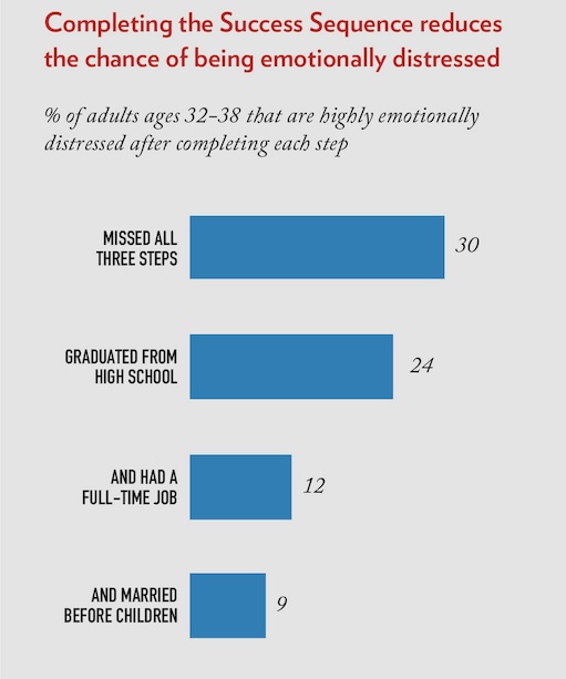
We find that the Success Sequence is strongly linked to better mental health among young adults. Our analysis of the Mental Health Inventory (MHI-5) in the NLSY97 demonstrates that the incidence of high mental distress at ages 32 to 38 drops dramatically with each completed step of the sequence. Millennials who completed all three steps are much less likely to be highly emotionally distressed by their mid-30s, compared with those who missed these steps (9% vs. 30%).
At the same time, there is a gender gap in mental distress among Millennials. Women are consistently more likely than men to report experiencing emotional distress. The gender gap is the largest among Millennials who missed all three steps of the Success Sequence (38% vs. 22%). But even among those who followed all three steps, women are still more likely than men to experience higher emotional distress (12% vs. 7%).
A racial gap also exists in mental distress among Millennials. White young adults who missed all three steps of the sequence by their mid-30s seem especially more likely to suffer from mental distress than other racial groups. Among this group, 38% of white young adults reported being highly emotionally distressed, compared with 23% of black and 26% of Hispanic young adults. This racial gap narrows with the completion of each step of the Success Sequence and is almost closed among young adults who have completed all three steps.
It is tempting to link better mental health to the financial success of the young adults who completed the Success Sequence, but the findings suggest that even after controlling for income, the sequence remains a significant factor in predicting your adult mental health. The odds of experiencing high emotional distress by their mid-30s are reduced by about 50% for young adults who have completed the three steps of the Success Sequence, after controlling for their income and a range of background factors, including gender, race, and family background.
Why does the Success Sequence contribute to better mental health? Further analysis suggests that the sequence is closely linked to family stability, which is key to mental well-being. Millennials who married before having children are more likely to have stable marriages. Among Millennials who followed this path, 73% are in intact families (married and never divorced) by their mid-30s, compared with only 30% of those who had children before or outside of marriage.
Furthermore, among Millennials who have been married and have children, those who became parents before marriage are about twice as likely to be divorced or separated by their mid-30s compared with their peers who married before having children (27% vs. 14%). Even after controlling for confounding factors like education, race, and family background, we find that marrying before having children is linked to a 32% decline in divorce among those who have ever married and have children.
Among the report’s other key findings:
Findings in this report are based on data from the Bureau of Labor Statistics’ National Longitudinal Survey of Youth, 1997 cohort (NLSY97).
NLSY97 follows the lives of a national representative sample of American youth (with black and Hispanic youth oversamples) born between 1980 to 1984. This cohort is also considered the oldest group of Millennials. The survey started in 1997, when the respondents (about 9,000) were ages 12 to 17. The interviews were conducted annually from 1997 to 2011 and biennially since then.
Respondents who stayed in Round 18 (N=6,734) are spotlighted in this report. They were in their mid-30s (ages 32-38) when surveyed in 2017 to 2018. The findings are weighted to reflect the characteristics of the overall population of American Millennials who were born between 1980 and 1984. The minimal sample size for the subgroup analysis is 100 unless otherwise noted.
To measure mental health, a five-item short version of the Mental Health Inventory (MHI-5) in NLSY97 was used. The items of the MHI-5 measure risks for suffering anxiety and depression, loss of behavioral or emotional control, and overall psychological well-being. Respondents were asked about how they felt during the previous month through a set of 5 questions, which include feeling nervous, feeling calm and peaceful, feeling downhearted and blue, being happy, and feeling so down in the dumps that nothing could cheer them up. Each question was rated on a 4-point scale: (1) All of the time, (2) Most of the time, (3) Some of the time, and (4) None of the time. The scores of the negative outcomes are reversely coded and scores of all five questions are combined into a mental health index range from 5 to 20. “Highly distressed” is coded as 1 standard deviation (S.D.) above the mean.
In the analysis of the Success Sequence, finishing high school and having a full-time job (working 35+ hours per week and 50+weeks a year) were measured when respondents were in their mid-20s. For more details about the methodology of the Success Sequence, please see the report The Millennial Success Sequence.
In this report, the term “Millennials” refers to adults born between 1980 and 1984, representing the oldest group of Millennials. The terms “Millennials” and “young adults” are used interchangeably, as are “mentally distressed” and “emotionally distressed.”
chapter 1: Navigating the Journey to Adulthood: Marriage, Parenthood, and Mental Health
The paths into adulthood for Millennials are more diverse than those of earlier generations. By their mid-30s, 45% of Millennials have married without first having a child, compared with about 70% of Baby Boomers when they were about the same age. Additionally, 35% of Millennials in this study have had children before or outside of marriage (compared to about 20% of Baby Boomers at the same age), and the remaining 20% of Millennials have never been married and are childless at ages 32 to 38.
Among young adults who are parents, there is almost an even split regarding the paths to parenthood. About 51% of Millennial parents in their mid-30s had children before or outside of marriage, while 49% took the path of getting married first before having children.
The order of marriage and parenthood matters for young adults’ health. Compared with their peers who had a child before marriage, Millennials who followed the path of “marriage first” are less likely to experience emotional stress and more likely to report being in great health and happy by the time they are in their mid 30s.1 For example, only 12% of Millennials who married before having a child report a high level of emotional stress, which is measured by a combination of mental health measures including depression, anxiety, and overall psychological well-being. In comparison, 19% of Millennials who had babies before marriage report a higher level of mental distress. Moreover, the group of Millennials who have never married and are childless report similar levels of mental distress as those who had babies before or outside of marriage.
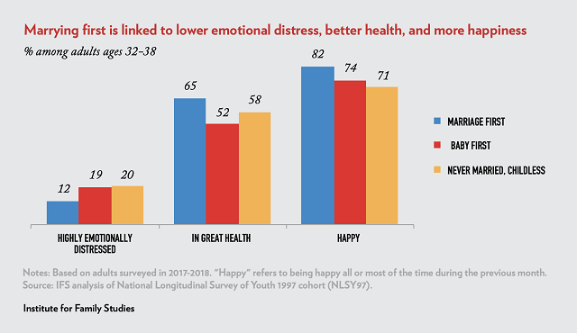
Marrying first is not only linked to a lower chance of emotional distress, but also to better general health and overall happiness. Millennials who married before having children are more likely than those who had children first to report being in great overall health when reaching their mid-30s (65% vs. 52%) and being happy all or most of the time (82% vs. 74%).
A closer look at different approaches to marriage and parenthood for Millennials in their 30s suggests that those who are currently married and had children after marriage have the lowest level of mental distress. Less than 10% of these adults reported high emotional stress, compared with 15% of Millennials who are married but either had children before marriage or are currently childless.
Divorce takes a toll on mental health. However, even among divorced young adults, the order of children and marriage is still linked to better mental well-being. Some 17% of divorced Millennials who became parents after marriage are highly stressed emotionally, compared with 26% of their peers who had children before marriage.
Millennials in their mid-30s who delay both marriage and parenthood (never married, childless) are equally likely to be emotionally stressed as their peers who have children but are not married. About 1 in 5 Millennials in these two groups experience high-level emotional distress, as do their peers who are divorced but do not have children.
These findings regarding mental health echo some of the results about Millennials’ family and financial status. We find that married Millennials who have children after marriage are most likely to be in the middle- and upper-income brackets (see more details in the Appendix). However, married and childless Millennials are better off financially than married Millennials who had children before marriage, yet the emotional stress levels in these two groups are similar. We also find that divorced and childless individuals are also better off financially than divorced Millennials who had children after marriage, but they have slightly higher rates of emotional distress. These findings suggest higher family income and better mental health do not always go handin-hand, especially when it involves children and marriage.
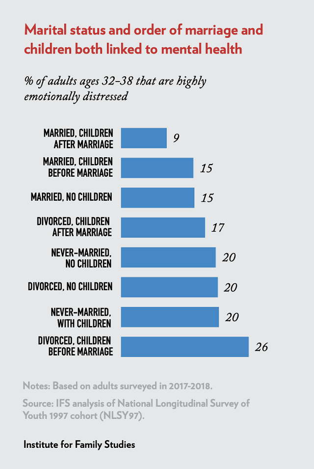
In addition to the order of marriage before having children, the Success Sequence includes two earlier steps: Getting at least a high school education and working full time. Our analysis finds that the Success Sequence is strongly linked to better mental health among young adults. For Millennials who complete all three steps of the sequence, the chance of being highly emotionally distressed is only 9% when they reach their mid-30s. In contrast, 30% of Millennials who missed all three steps are in mental distress at this life stage, and those who completed the education and work steps but didn’t marry before having a child are also more likely to be highly distressed (12%) when they are in their mid-30s.
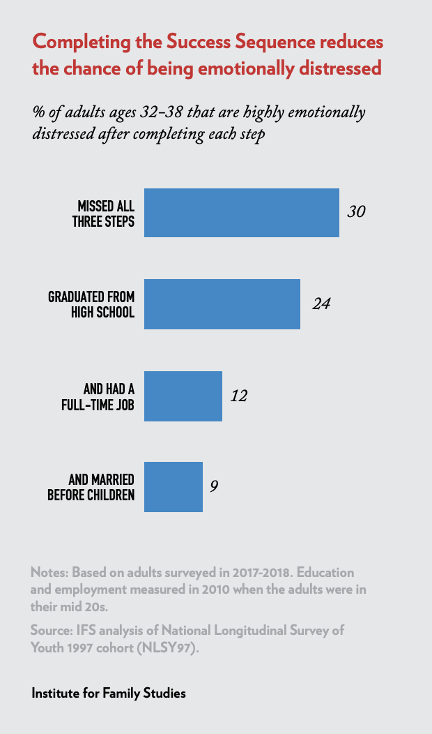
It may seem logical to attribute better mental well-being to the financial success of young adults who followed the Success Sequence, but the findings suggest that even after controlling for income, the sequence remains a significant factor in the mental health of young adults. The odds of experiencing high emotional distress by their mid-30s are reduced by about 50% for young adults who have completed the three steps of the sequence, after controlling for a range of background factors including family income, education, gender, and race (see Table 1 in the Appendix for details).
To see exactly how the order of marriage and parenthood plays out for Millennials, we also looked at the impact of the Success Sequence among Millennials who have had children (about 70% of Millennials have had children by age 32 to 38). The findings are identical: Millennial parents who missed all three steps of the sequence are much more likely than others to experience mental distress. In contrast, the mental distress level is much lower, around 7%, among Millennial parents who have completed all three steps of the sequence (see figure in Appendix for more details).
Millennial women are consistently more likely than men to be emotionally distressed. Overall, about 19% of Millennial women in their mid-30s report high emotional stress, compared with 13% of Millennial men. Among Millennial women who missed all three Success Sequence steps, 38% are highly emotionally distressed at ages 32 to 38. The share is 22% for Millennial men who missed all three steps by their mid-30s. With the completion of each step of the Success Sequence, the emotional stress level generally goes down for both Millennial men and women, but the gender gap remains. Even among Millennials who have followed all three steps, women are still more likely than men to experience high emotional stress (12% vs.7%).
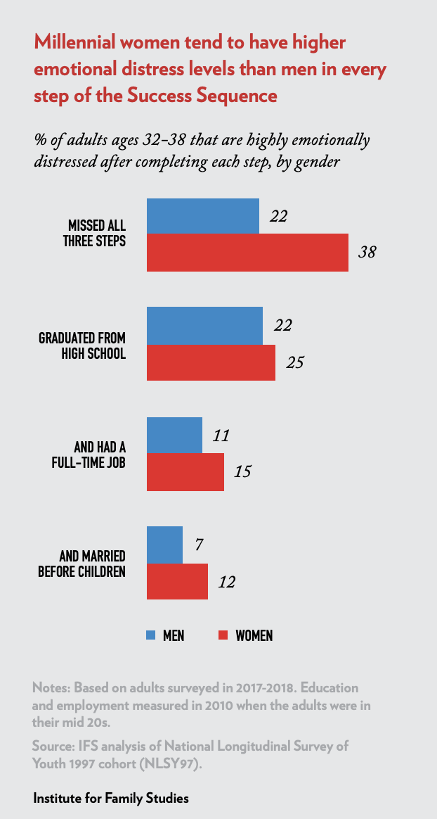
A similar gender gap also exists among Millennials who have children. Among Millennial parents who missed all three steps of the Success Sequence, 36% of mothers and 19% of fathers are highly emotionally distressed by their mid-30s. The gap is significantly reduced but remains among Millennial parents who have completed all three steps of the Success Sequence: only 5% of Millennial fathers and 10% of Millennial mothers who followed the sequence experience high mental distress by their mid-30s.
These findings are in line with longstanding patterns from psychiatry that women are more likely to suffer from anxiety or depression. Several potential reasons have been offered as to why women are more prone to emotional distress, including the fact that women experience more hormonal fluctuations that can trigger clinical depression or anxiety. For example, women are prone to particular forms of depression or anxiety that are specifically triggered by these hormonal changes, including premenstrual dysphoric disorder, postpartum depression, or postmenopausal depression or anxiety, whereas men do not experience these conditions.
Looking at the different family paths Millennial men and women have taken, we find that overall, married women who have children after marriage enjoy better mental health than other women, with only 12% of them experiencing high emotional stress in their mid-30s. On the other hand, divorced Millennial women who had children before marriage have the highest levels of mental distress by their mid-30s. About 1 in 3 divorced Millennial women who had children outside of marriage are highly distressed.
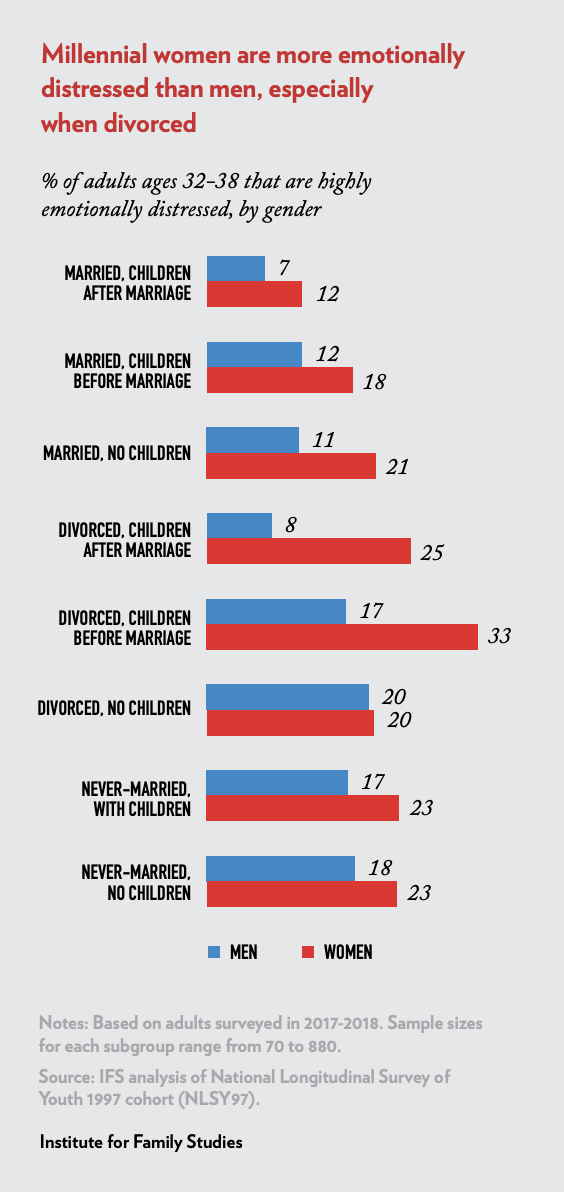
In contrast, divorced Millennial women who had children after marriage suffer less emotional distress. About 1 in 4 of these women reported being highly emotionally distressed. This is similar to the emotional distress levels among never-married women (with or without children).
Young men’s emotional distress levels are lower overall than that of young women in most of these different family paths, except among young adults who are divorced but childless. An equal share of young men and women (20%) in this group experience a high level of emotional distress, which represents the highest level of emotional distress among Millennial men in their mid-30s. Millennial men who are currently married and have children after marriage experience the lowest levels of mental distress. Interestingly, divorce doesn’t take a heavy toll on young men who are divorced but have children after marriage. Only 8% of men in this situation experience high emotional distress, which is similar to the rate for men who are married and had children after marriage.
In contrast to the financial success story presented in the previous IFS report on the Success Sequence, where white Millennials were consistently less likely than black and Hispanic Millennials to be in poverty, white Millennials do not have an advantage over other young adults when it comes to emotional well-being. In fact, they are generally more likely than other races to experience emotional distress.2 Among young adults who have missed all three steps of the sequence by the time they are in their 30s, white young adults are much more likely to report that they are highly emotionally stressed (38%) compared with black young adults (23%) and Hispanics (26%), despite the fact that white young adults in this situation are much less likely to be in poverty than the other two groups.
With completion of each step of the Success Sequence, the racial gap narrows. For Millennials who followed all three steps, the share of highly emotionally stressed young adults drops to 9% for whites, 8% for bBlacks, and 9% for Hispanics. The racial gap in emotional well-being is almost closed.
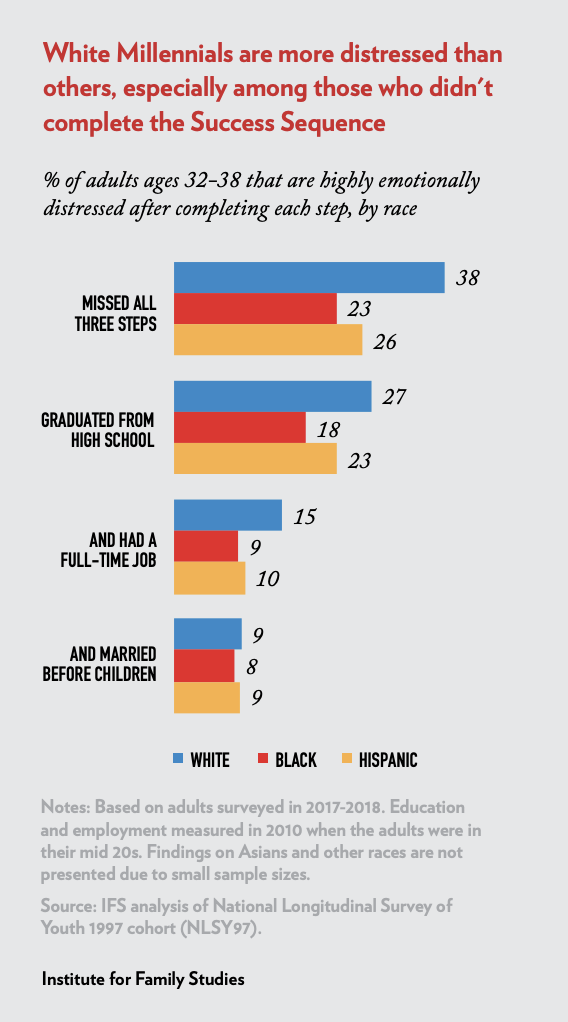
Previous studies on Millennial health showed that Millennials in majority black and Hispanic communities have significantly lower rates of depression than those in majority white communities, with some hypothesizing that these differences could be due to under-diagnosis in communities of color. Our analysis of NLSY data support a lower rate of symptoms of depression and anxiety among black and Hispanic individuals. Notably, the self-report nature of this data suggests that lower rates of depression and anxiety symptoms among black and Hispanic individuals may not be due to underdiagnosis and that other factors may be at play.
Taken together, the Success Sequence’s link to both economic success and emotional well-being suggests that following the sequence offers a clear path to closing the racial gap, not only in terms of economic well-being but emotional well-being as well.
The Success Sequence benefits Millennials’ mental health not only through the financial success it brings but also because it is linked to another important factor in mental health: family stability.
Millennials who followed the sequence of marrying before having children are more likely to have stable marriages. Among Millennials who married before having children, 73% are in an intact family (married and have never been divorced) by the time they are in their mid-30s, compared with only 30% of Millennials who had children before or outside of marriage. Furthermore, among Millennials who have been married and have children, those who became parents before marriage are about twice as likely to be divorced or separated by the time they reach their mid-30s, compared with their peers who married before having children (27% vs. 14%).
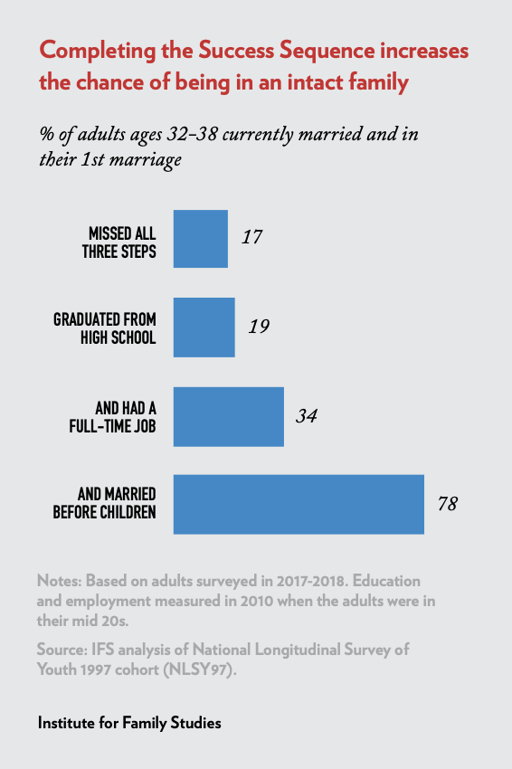
Following all three steps of the Success Sequence—getting at least a high school education, working full-time, and marrying before having any children—leads to much higher family stability by the time Millennials reach their mid-30s. Close to 80% of young adults who followed this path are married and have never divorced, compared with 34% of young adults who missed the step of marrying before children, and 17% of young adults who missed all three steps.
Moreover, after controlling for a range of sociodemographic factors, young adults who followed the three steps of the Success Sequence are four times more likely to be living in an intact family in their 30s compared with their peers who didn’t follow the sequence. The fact that family stability is key to mental health is supported by multiple lines of research. For children, parental divorce is a large and consistent risk factor for anxiety, depression, and substance use. Family stability (as in marital stability without divorce) has repeatedly been shown to lead to better financial and educational outcomes for children, which in turn reduces the risk of mental health problems.3 Another key way that family stability may mediate improved mental health outcomes for children is by protecting them from physical and sexual abuse, which greatly increase the risk of psychiatric problems.4 Overall, children from families with married biological parents are three to 10 times less likely to experience physical abuse compared to children in step-families or in households headed by single parents with or without romantic partners; they are also five to 20 times less likely to experience sexual abuse.5
Family stability is also important for the mental health of adults. Reports based on large and nationally representative surveys have shown that both men and women who marry and remain married have lower rates of depression, anxiety, suicide, and suicide attempts compared to those who are single, widowed, or divorced.6 These findings parallel the conclusions of this research brief.
There are many contributing factors to mental health, but family stability is clearly a major factor. The findings of this report are in line with decades of research from psychology showing that relationships are fundamental to human happiness and well-being. Furthermore, among the many relationships that affect us, marital relationships tend to have the greatest bearing on our emotional (as well as physical) health.
The mere act of being married raises the probability that someone is very happy by a substantial amount. In a prior analysis of data (1972-2021) from the General Social Survey, 37% of those who were married reported they were very happy compared to 18% who were single, widowed, or divorced.
There are many potential ways that marrying before having children favors greater relationship stability compared to when the sequence is reversed. Divorce is one measurable indicator.
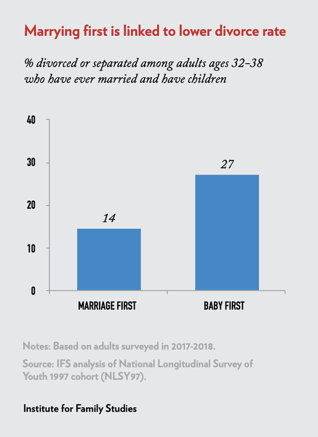
Divorce is a major stressor in life, and it is linked with an increased risk of anxiety, depression, and alcohol abuse, along with other negative mental health outcomes. When we limit the analysis to Millennials who have been married and have children, a clear pattern emerges regarding the order of marriage and having children and family stability. Millennials who became parents before getting married are about twice as likely to be divorced or separated by the time they are in their mid-30s, compared with their peers who married before having children (27% vs. 14%).7 Even after controlling for confounding factors like education, race, and family background, we find that marrying before having children is linked to a 32% decline in divorce among those who have ever married and have children.8
Both groups are married with children. But what explains why the group who had children before marriage is more likely to experience divorce than those who had children after they were married? Many factors could be at play. Couples who have children before marriage may not have fully established the foundation of their relationship, such as commitment and communication, which often leads to increased marital strain. Additionally, the stressors associated with unplanned pregnancies and early parenthood may exacerbate existing relationship challenges.
Moreover, our findings suggest that Millennials who become parents before marriage tend to have children at an earlier age than those who marry first (with a median age for first birth of 21 vs. 28), but they marry later than the “marriage first” group (at 26 vs. 24). With an extended gap between first birth and marriage, it is possible that some Millennials who follow this path may not necessarily marry the parent of their children, further complicating family relationships. These complexities in family dynamics could contribute to the increased likelihood of divorce among couples who had children before marriage.
The Success Sequence—completing at least a high school education, securing full-time employment in their 20s, and marrying before having children—not only offers a promising path for young adults to achieve economic success but is also closely linked to emotional and mental well-being. Moreover, the ways in which the Success Sequence contributes to mental health are not limited to financial success but also to the higher levels of family stability associated with following this path.
Our findings demonstrate that young adults who’ve followed the three steps of the Success Sequence experience significantly better mental health by their mid-30s compared with those who have not. This is true even after accounting for various background factors such as income, gender, and race. The odds of experiencing high emotional distress are reduced by about 50% for those who have completed each step.
Family stability emerges as a crucial factor in the mental well-being of Millennials. Those who marry before having children are more likely to maintain intact families, with 73% remaining married by their mid-30s. In contrast, those who have children before marriage face much higher rates of divorce and separation. The extended gap between first birth and marriage in this group often complicates family relationships, potentially leading to greater family instability and subsequent mental health challenges.
Given the mental health crisis among Millennials and young adults, it is important for young people to understand what patterns are more likely to help them form families that lead to better mental health. Unfortunately, a variety of factors in contemporary culture have made it more difficult for young people to form stable marriages and families.
One factor is that marriage is less likely to be valued than work or education. A 2023 Pew Research Center report noted that 88% of parents agreed it was “very” or “extremely” important for their children to have an enjoyable job, and 41% said it was very or extremely important for their children to graduate from college, whereas only 20% of parents attached the same level of importance to their children getting married. These goals run in contrast to decades of sociological data that conclude a good marriage is more important to well-being than other factors, including career.9
This mismatch between those goals we tend to prioritize and what actually leads to enduring well-being occurs on an individual level as well. Predicting how we are going to feel in a given circumstance is known as affective forecasting. Humans make such predictions every day without thinking, and these predictions shape life priorities. Surprisingly, humans are relatively poor judges of what leads to enduring well-being.
Psychological science has repeatedly shown that relationships are the most important factor for well-being and happiness.10 The most important relationship is with one’s romantic partner or spouse. Helping young people understand the importance of relationships to well-being is critical to helping them prioritize marriage.
Today’s young adults receive ample training and guidance in education and career, but when it comes to getting married and having children, most people “just wing it.” Among the key components of the Success Sequence—education, work, marriage, and children—training and guidance on healthy marriages and family life are severely lacking.
As we suggested in previous reports, we should teach the Success Sequence in schools and promote it via public campaigns. For those who care about both the economic and emotional well-being of today’s young adults—policymakers, educators, business and community leaders, influencers, as well as parents—it is time to help young adults understand how following each step in the Success Sequence will increase their chances of a financially and emotionally healthy life.
The “Marriage first” group includes those who had children after marriage, regardless of their current marital status, as well as those who are currently married but do not have children. The “Baby first” group includes those who had children before marriage or outside of marriage, regardless of their current marital status.
Overall, 17% of white Millennials in their mid-30s reported high emotional stress, compared with 14% of Black Millennials, 14% of Hispanic Millennials, and 11% of Asian Millennials, according to NLSY97 data.
David Blankenhorn. Fatherless America: Confronting Our Most Urgent Social Problem. (New York City: Harper Perennial, 1996); David Popenoe. Life Without Father: Compelling New Evidence That Fatherhood and Marriage Are Indispensable for the Good of Children and Society. (Cambridge: Harvard University Press, 1999). Also: Melissa Kearney. The Two-Parent Privilege: How Americans Stopped Getting Married and Started Falling Behind. (Chicago: University of Chicago Press, 2023).
Jutta Lindert, et al., “Sexual and physical abuse in childhood is associated with depression and anxiety over the life course: A systematic review and metaanalysis.” International Journal of Public Health 59, no. 2 (2014): 359-372.
Felicitas Auersperg, et al., “Long-term effects of parental divorce on mental health: A meta-analysis.” Journal of Psychiatric Research 119 (2019): 107-115. Brad Wilcox. Get Married: Why Americans Must Defy the Elites, Forge Strong Families, and Save Civilization. (New York City: HarperCollins, 2024).
Office of the Assistant Secretary for Planning and Evaluation. The Effects of Marriage on Health: A Synthesis of Recent Research Evidence. (Washington, DC: U.S. Department of Health and Human Services, June 2007). Sohrab Iranpour, et al., “The trend and pattern of depression prevalence in the U.S.: Data from National Health and Nutrition Examination Survey (NHANES) 2005 to 2016.” Journal of Affective Disorders 298, part A (February 2022): 508-515. W. KyungSook et al., “Marital status integration and suicide: A meta-analysis and meta-regression.” Social Science & Medicine, 197 (2018): 116-126. T.J. Bommersbach, “National trends of mental health care among US adults who attempted suicide in the past 12 months.” JAMA Psychiatry 79, no. 3 (2022): 219-231.
Marital status was measured at ages 32 to 38, accounting for multiple divorces and remarriages.
The regression model includes work status and whether the respondents lived with both of their parents during their teenage years.
Op. Cit, Wilcox. Get Married.
Robert Waldinger and Marc Schulz. The Good Life: Lessons from the World’s Longest Scientific Study of Happiness. (New York: Simon & Schuster, 2023). M.E.P. Seligman. Flourish: A Visionary New Understanding of Happiness and Well-being. (New York: Atria Books, 2011).
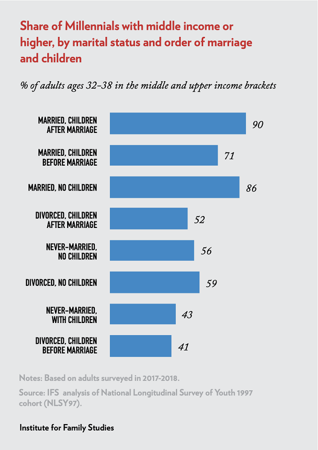
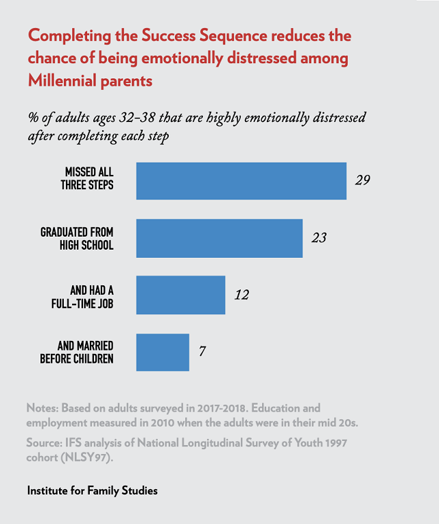
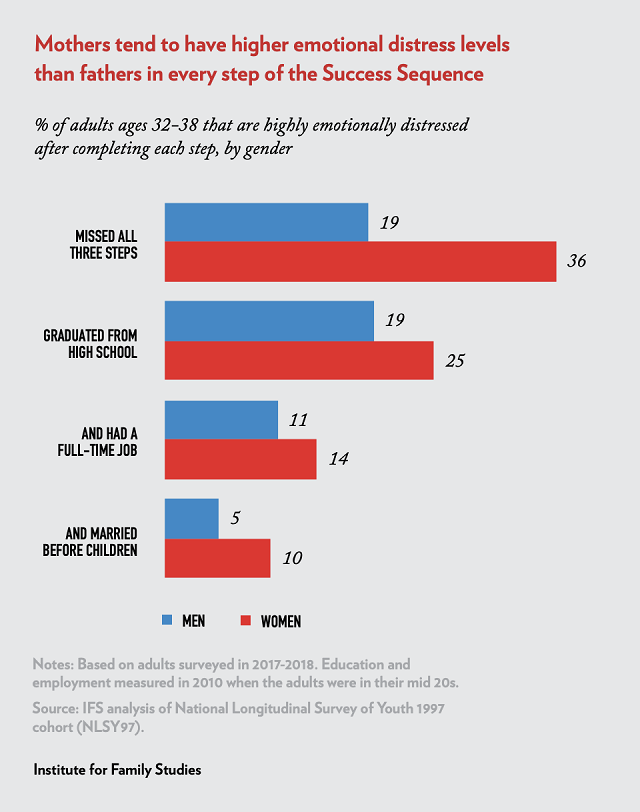
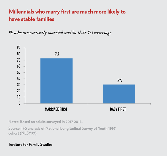
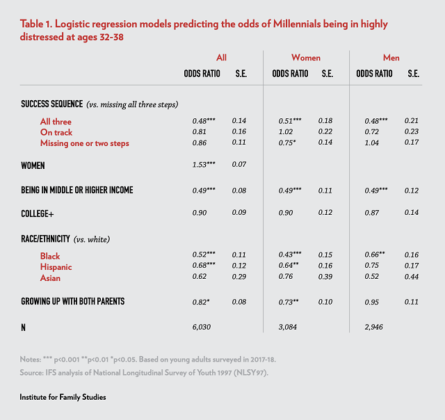
About the Authors
Wendy R. Wang, Ph.D. is Director of Research at the Institute for Family Studies. She has published widely on topics including marriage, gender, work, family, happiness, and well-being. Dr. Wang is a former Senior Researcher at Pew Research Center and the lead author of the Pew Research Center report, Breadwinner Moms, among other Pew reports.
Samuel T. Wilkinson, MD, is Associate Professor of Psychiatry at the Yale School of Medicine and the Associate Director of the Yale Depression Research Program. His research specializes in innovative treatments for depression, including novel pharmacological and neuromodulation techniques. Dr. Wilkinson is also the author of the book Purpose: What Evolution and Human Nature Imply about the Meaning of Our Existence.
Acknowledgements
The authors would like to thank IFS senior fellow Brad Wilcox for his insights and substantive feedback on this report. We would also like to thank Alysse ElHage for editing the report and Brandon Wooten for its design.

May 2025 | by John Iceland, Jaehoon Cho
May 2025
by John Iceland, Jaehoon Cho
This research brief focuses on differences across household types in income, non-income resources, such as wealth, and demographic and socioeconomic characteristics, such as age and education.
Download PDFMarried-couple households are more affluent, less likely to be poor, and experience fewer hardships than other types of households, such as single-parent families or people living on their own. This research brief explores why, focusing on differences across household types in income, non-income resources, such as wealth, and demographic and socioeconomic characteristics, such as age and education.
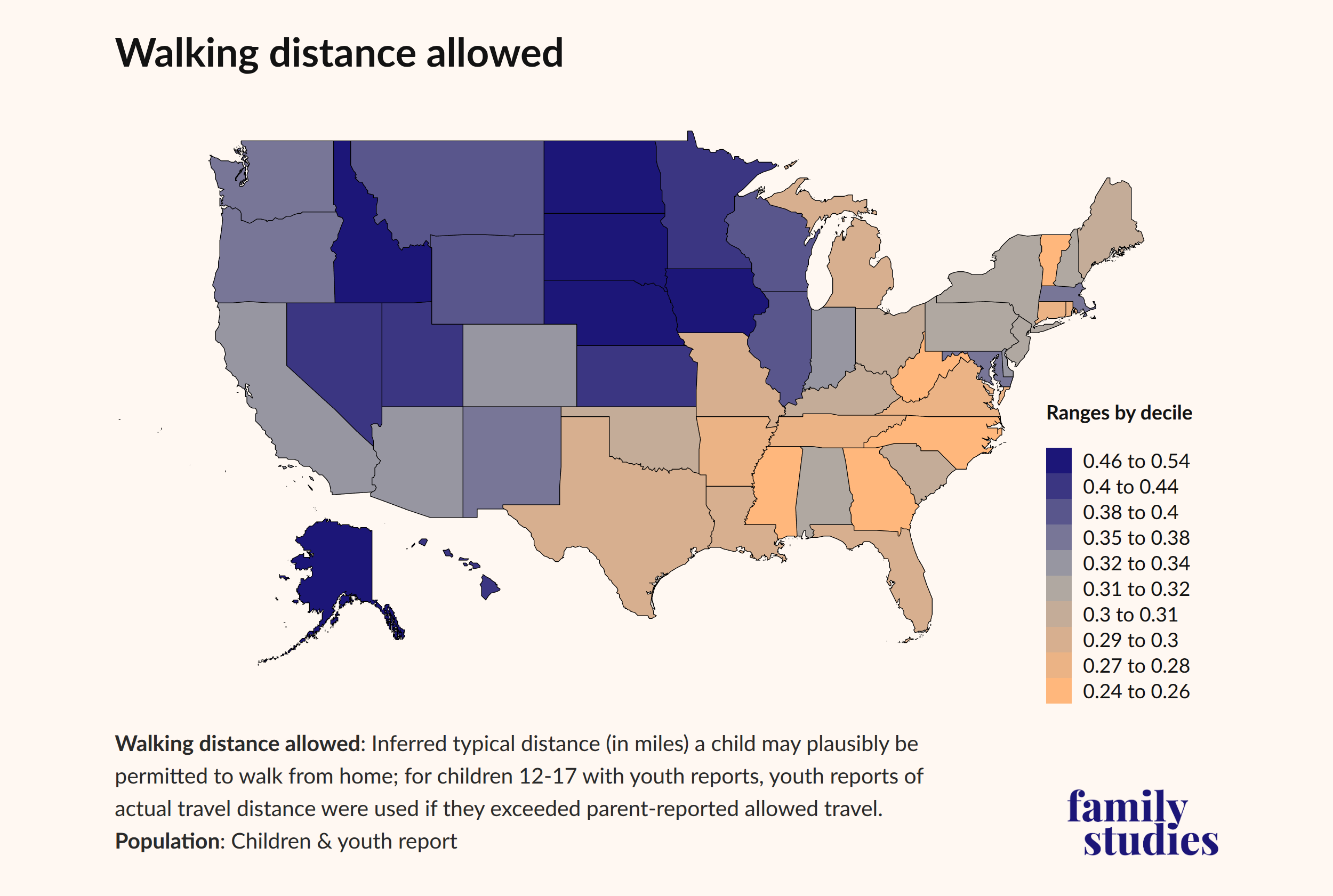
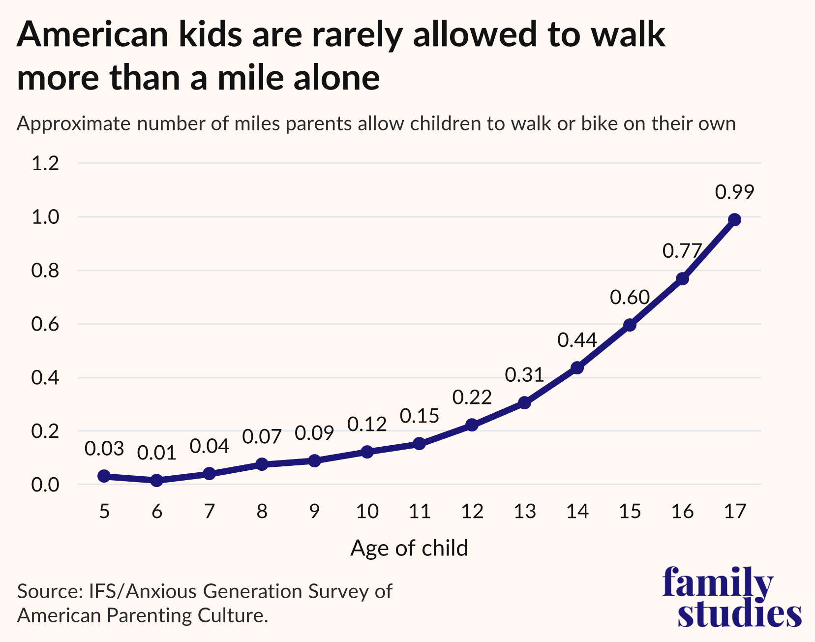
In our recent study, published in Demographic Research, we find that married-couple households experience fewer hardships than other households while single-parent families with children experience the most. Other household types, such as cohabiting couples and people living alone, fall in between. The biggest reason for the married-couple advantage is wealth—married couples often have more savings and assets to fall back on. Income also plays a significant role, followed by demographic and socioeconomic characteristics.
In short, the income- and wealth-building capacity of married-couple households are important for helping them avoid hardships. Meanwhile, a more moderate portion of the married-couple household advantage reflects the selection of more fortunate demographic and socioeconomic groups into marriage—for instance, people with higher levels of education are more likely to marry than others.

May 2025 | by Erik Randolph
May 2025
by Erik Randolph
A two-part IFS policy brief on how to eliminate marriage penalties from the tax code and safety-net programs.
Download PDFThe U.S. individual income tax structure and the safety-net assistance system exact financial penalties on married couples, which worsen when children are in the family. The effect of these penalties is the opposite of what public policy should be. Research has established that society benefits immensely from stable and healthy marriages. This policy brief is divided into two sections. Section 1 focuses on the U.S. Tax Code and restoring the income tax to its primary purpose, while eliminating the marriage penalty. Section 2 presents a way for Congress to eliminate marriage penalties from safety-net programs.

An IFS research brief on the fertility-boosting benefits of expanding the Child Tax Credit (CTC).
Download PDFWhat would happen to American fertility if the child tax credit were appreciably increased? Many are skeptical of the influence of cash transfers on fertility, but that skepticism is misplaced. Cash-for-kids works. It is relatively cost-effective, and its fertility effects help families achieve their own stated family goals. The pronatal outcomes of an increased child tax credit are a good reason to support such an investment.
Key Findings:

April 2025 | by Grant Martsolf, Brad Wilcox
April 2025
by Grant Martsolf, Brad Wilcox
This IFS report examines family formation among working-class men, defined as men without college degrees, within the context of distinct employment environments. We also examine differences in married family formation rates between working-class and college-educated men, and the extent to which these differences might be explained by differences in pay, benefits, and stability.
Download PDFGrant Martsolf, Brad Wilcox, Good Jobs, Strong Families. How the character of men's work is linked to their family status (The Institute for Family Studies, Penn’s Program for Research on Religion and Urban Civil Society (PRRUCS), 2025)
Media Coverage
John DiIulio, "The best natalist policy: good jobsThe makings of a second Baby Boom," UnHerd, May 26, 2025
Chris Bullivant, Grant Martsolf, Brad Wilcox, "Is the collapse of blue-collar marriage a foregone conclusion," The Washington Examiner, April 30, 2025
Grant Martsolf, "Good jobs, strong families in working-class America," Family Studies, April 29, 2025
Introduction
Over the last half century, the U.S. economy has shifted, moving away from manufacturing and towards being an information and service economy. The mid-1980s, for instance, were punctuated by news of the closures of major steel manufacturers, including Homestead Works, Aliquippa Works, and Duquesne Works in Pittsburgh, PA, and Republic Works in Youngstown, OH. The closures were part and parcel of a period of massive deindustrialization. Between 1984 and 2004, the U.S. economy lost between 6 and 7 million manufacturing jobs that provided reliable and high-paying employment with good benefits for millions of working-class Americans.
The move away from manufacturing had a significant impact on America’s working class. Real wages of the median Americans with a high school diploma or less (a common measure of “working class”) declined by 11% between 1979 and 2019, while those of the median worker who had finished college increased by 15 percent. Many industrial communities, especially across America’s “Rust Belt,” experienced significant disinvestment and fell into blight. These economic shifts, both in the Rust Belt and nationwide, took a devastating toll. They pushed working-class men’s labor force participation down and led to declines in religious and secular expressions of community life in areas hit hardest by deindustrialization. Families not only broke apart but failed to form. In the wake of this economic dislocation and social breakdown, deaths of despair—that is, deaths from drug overdoses, suicides, and alcoholism—surged among working-class women and especially men.
The transformation of the American economy has been especially impactful on working-class men. As manufacturing receded, employment in service industries surged, especially in healthcare, financial, and information services. Many of these service jobs require a college degree. And most of the significant growth in jobs that do not require a college degree has been concentrated in industries and occupations that are female dominated. Since 1990, the healthcare industry alone has added roughly 9 million jobs to the US economy. Nearly 80% of Americans who do not have a college degree and work in healthcare are women.nbsp;In fact, declines in real wages for working-class workers were concentrated among men; working-class women have seen their real wages rise since 1979.
Over this same period, Americans have also experienced a significant reduction in marriage and family stability. Since 1970, the marriage rate has fallen by more than 60% to the point where only about 1 in 2 adults are married. Declines in marriage and family stability have been especially precipitous for working-class Americans since 1980. For instance, only 39% of non-college-educated Americans ages 18-55 are married, compared to 58% of college-educated Americans.
Our hypothesis in this Institute for Family Studies (IFS) report is that the nature and character of work play a key role in affecting male marriageability. We contend that features of work like job stability, predictable hours, good benefits, and high pay help men to flourish and, in turn, elevate their appeal as husbands. Moreover, we note that class divides in marriage today are driven in part by differences in the character of work, with college-educated men generally benefiting, in terms of marriage and family formation, from jobs that are more stable, predictable, higher status, and remunerative. But we also suspect that the character of work varies among working-class men themselves, such that some jobs among working-class men are more likely to facilitate marriage and family formation than others.
In this report, we examine family formation among working-class men, defined here as men without college degrees, within the context of distinct employment environments. We also examine differences in married family formation rates—measured here in terms of being married with children at home—between working-class and college-educated men, and we investigate the extent to which these differences might be explained by differences in “good job” variables—primarily differences in pay, benefits, and stability. We then explore differences in the rates of married family formation among working-class men by industry and estimate the extent to which differences across industries are explained by the same “good job” variables. We conclude with a discussion of how public policies might better support working-class men in their jobs to improve their family prospects.
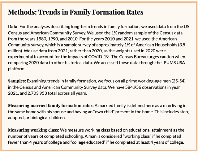
Part 1: Family Formation Among Working-class Men
Trends in family formation rates
In this section, using historical Census data from 1980-2021, we discuss recent family formation trends among working-class men. Working class throughout this report is operationalized as completion of less than a college education. Here, college education is defined as completion of at least four years of college. Importantly, this is slightly different than the operationalization of “working class” because the measures of educational attainment in historical Census data are slightly different from the CPS data used in subsequent analyses.
There is ample evidence that college-educated Americans are more likely to get married, stay married, and avoid having children out of wedlock. This is partly because more educated men and women have more stable incomes, more shared assets, greater civic supports for their marriages, and networks that are dominated by married peers, as Wilcox argued in Get Married.
However, this has not always been the case. In fact, before the 1980s, men who did not complete college had higher rates of married family formation compared to those who did complete college. In our analysis of Census data, we found that in 1980, 59% of all prime working-age men (ages 25-55) who did not complete college were married with children living in their homes, compared to 55% of men who did complete college.
Over the course of the next 40 years, all men in America were increasingly less likely to be married and living with children. By 2021, only 37% of prime working-age men were married living with children compared to 58% in 1980 (Figure 1). But the overall decline in married family formation was more significant for men who had not completed college. Over the last 40 years, men who had not graduated from college were now actually less likely than college-educated men to be married and living with their own children. By 2021, 34% of non-college-educated, prime working-age men were married and living with their own children compared to 44% of college-educated men.
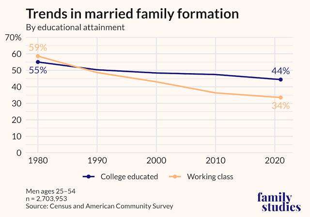
We examine more closely family formation rates among working-class men ages 25-55 in 2021 (Table 1). We found that working-class men (33.50%) were much less likely to be married with children living in their homes compared to college-educated men (44.39%). At the same time, they were much more likely to cohabit with children in the home (3.44% vs. 0.93%) and to be living with no partner and without children (41.36% vs. 31.83%).
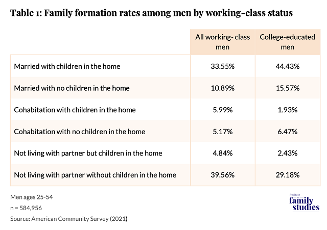
Part 2: Examining Married Family Formation by Class and the Impact of Good Job Variables
Married family formation rates by class
This section compares all college-educated versus working-class men. We are interested primarily in the links between class, workplace environment, and family status. For this analysis, we use data from the Current Population Survey from years 2021-2024. We used regression models to estimate predicted probabilities of having a married family by education, which we view as a proxy for class. In our sample of 113,656 prime working-age men, we find that working-class men were 8 percentage points less likely than college-educated men to be married and living in the home with their children (Table 2). Regression coefficients used to produce these adjusted rates are shown in Appendix Table A3.
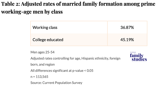
Mediation of differences across class by good job variables
We then examine the extent to which differences in married family formation across classes might be explained by differences in the types of jobs that working-class and college-educated men hold (i.e., good job variables). To determine the extent to which differences could be explained by good job variables, we performed a mediation analysis using the Barron and Kenney framework. To do this, we must first establish that good job variables are associated both with class and married family formation. If so, we can test the mediation impact of good job variables on marriage formation rates.
We first compare good job variables across working-class and college-educated men. We find significant differences across classes. Most notably, a majority of college-educated men (61.33%) make a “good wage” (i.e. >$60,000 per year) compared to a minority of working-class men (26.18%). College-educated men are also much more likely to have stable jobs. They are also about 20 percentage points more likely than working-class men to have employer-sponsored health benefits. They are much more likely to have all three good job characteristics at their current employer (Table 3). Regression coefficients used to produce these adjusted rates are shown in Appendix Table A4.
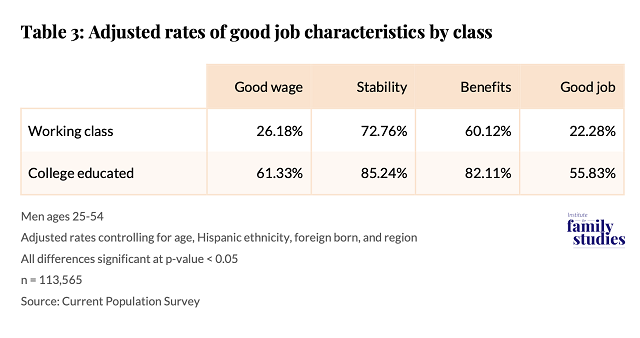
These good job characteristics are also correlated with married family formation rates. We find that those with good job characteristics are much more likely to be married family men. Those with all three of these good job characteristics are 17 percentage points more likely than those who do not have all three of these characteristics to have a married family (Table 4). Regression coefficients used to produce these adjusted rates are shown in Appendix Table A5.
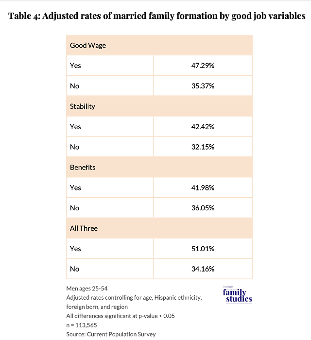
Finally, we examined the extent to which the good job variables mediate the relationship between class and family formation rates. Table 5 shows that good job variables are in fact a significant meditator between class and married family formation. These good jobs variables explained nearly 80% of the adjusted differences in married family formation rates by class (Table 5). This is a striking finding. It underlines the ways in which the character of college-educated men’s jobs probably helps explain why they are markedly more likely to get and stay married than working-class men. Of course, we cannot determine the direction of causality here. All that we can say is the class divide in marriage between college-educated and working-class men is closely tied to the class divide in the character of men’s work. Regression coefficients used to produce these adjusted rates are shown in Appendix Table A3.
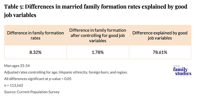
Part 3: Examining Married Family Formation by Industry Among Working-class Men
Married family formation rates by industry
Patterns of married family formation for working-class men differ by employment industry. In this section, we focus exclusively on men who report having worked during the observation year. Only those who worked at some point during the observation year will have data on primary industry. For this analysis, we use data from the Annual Social and Economic Supplement (ASEC) of the Current Population Survey (CPS) from years 2021-2024. Table 6 indicates wide variation across industries in terms of the rates of married family formation for working-class men. The highest married family formation rates among working-class men are in the armed forces and public order and safety, followed by trucking, construction, and maintenance and repair. The high rates of married family formation in the armed forces are consistent with earlier research indicating that the armed forces continue to support marriage and family life. Surprisingly, manufacturing falls in the middle. By contrast, the lowest shares of married family formation for working-class men are in healthcare, retail, and food and hospitality. Regression coefficients used to produce these adjusted rates are shown in Appendix Table A6.
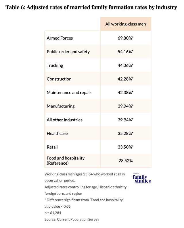
Mediation of differences across industries by good job variables
For working-class men, there is clearly variation between industry and family structure. How much are differences in married family formation rates across industries linked to differences in “good job” variables, including pay, health insurance benefits, and stable employment? In this section, we take up this question.
To determine the extent to which differences could be explained by these good job variables, we again perform a mediation analysis using the Barron and Kenney framework. In examining the relationship between industry and good job variables, we find that some industries have more good job characteristics than others, as Table 7 indicates. Public order and safety, armed forces, trucking, and manufacturing have higher rates of good wages, while retail, food and hospitality, and maintenance and repair have significantly lower rates. Likewise, there were significant differences in job stability across industries with public order and safety, manufacturing, armed forces, and trucking enjoying the highest rates of stability, while food and hospitality had the lowest. In terms of benefits, public order and safety, manufacturing, trucking, healthcare, and, especially, armed forces had the highest rates of uptake of employer sponsored health insurance, while construction, food and hospitality, and maintenance and repair had the lowest. Again, our results here are indicative of the marriage- and family-friendly character of military jobs. Overall, public order and safety, manufacturing, construction, and trucking had the highest rates of all three good job characteristics, while retail, maintenance and repair, and especially food and hospitality had the lowest rates. We show the detailed regression results used to generate these adjusted rates in Appendix Table A7.
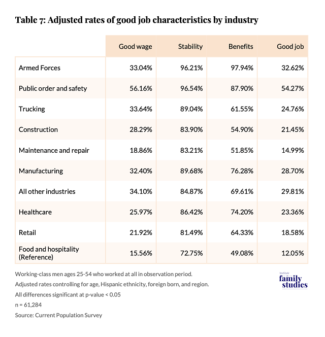
We also examined the relationship between family formation rates and good job variables within the Part 3 sample. Table 8 indicates that each of the good job variables is consistently correlated with higher rates of married family formation for working-class men. Regression coefficients used to produce these adjusted rates are shown in Appendix Table A8.
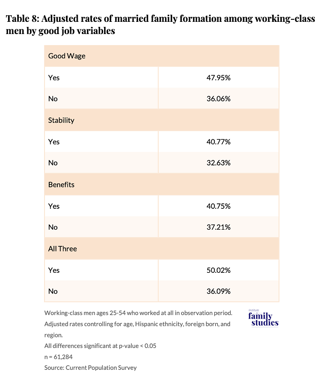
Finally, we examined the extent to which the good job variables mediated the relationship between industry and married family formation rates. Table 9 shows that good job characteristics are in fact a mediator between industry and married family formation for most sectors of the economy, but the amount of difference in married family formation rates explained by good job characteristics varies significantly across industries. The good job characteristics explain between 8-44% of the difference in married family formation between each of the industries compared to the food and hospitality industry. Regression coefficients used to produce these adjusted rates are shown in Appendix Table A6.
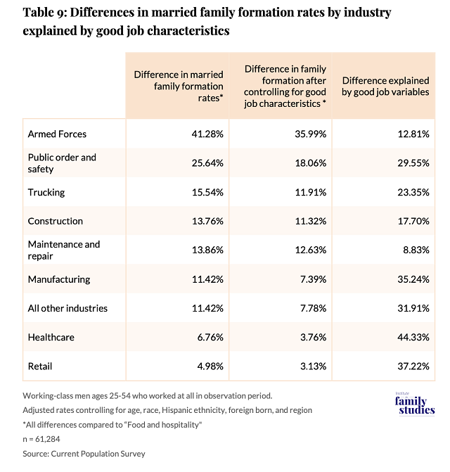
Conclusion
This Institute for Family Studies report suggests that both the nature and character of men’s work play a major role in determining whether men marry and form families. One big reason that working-class men are less likely to form married families seems to be that they have lower quality jobs—jobs marked by less income, less stability, and lower benefits. These findings must, however, be interpreted with caution. We do not show a direct causal relationship between good jobs and married family formation here, though we do show that having a good job is linked to men’s marital and family fortunes. To wit: prime-aged men with good jobs are markedly more likely to be married with children than men in lower quality jobs. So, consistent with the broader literature on work, men, and marriage, we think that access to good jobs increases the odds that men marry and form families.
Moreover, we document that differences in job quality help explain, statistically, almost 80% of the differences in the married family formation rates between working-class and college-educated men. This is a striking finding. Class differences in men’s work are clearly tied to class differences in marriage and family formation. The clear implication here is that men are more likely to be married with children when they are well paid, their jobs are stable, and their benefits are good.
Moreover, among working-class men, the findings of this IFS report suggest that having a good, working-class job appears to help explain differences among working-class men in married family formation rates across industries. More concretely, the fact that sectors like public order and safety, trucking, and manufacturing often have higher pay, greater job stability, or better benefits may help explain why men in these jobs also have comparatively high levels of married family formation. Undoubtedly, the good job characteristics that are more likely to define these sectors help explain why men who serve in these jobs are the working-class men most likely to be married with children.
In our analysis of industries and married family formation among working-class men, our good job variables do not explain all the difference in married family formation rates across industries among working-class men. There are likely other differences in job characteristics across the industries that we could not measure that may influence married family formation. We were particularly struck by the exceptionally high rates of family formation for men serving in the armed forces, which are not completely explained by our specific measures of good job characteristics. It may be that the military has a culture that is more friendly to marriage and family formation, or that the extra housing benefits (which we did not measure) extended to married service members make marriage more attractive to men in the military.
We also observed that healthcare, retail, and food and hospitality had lower levels of married family formation. This could be because many of these jobs are marked by erratic and unpredictable schedules that make it difficult to forge a strong and stable family. Many cities and states have attempted to alleviate this problem by legislating predictable schedules with some success.Some sectors—like food and hospitality—may also be associated with a culture of late nights and substance use that is not conducive to forming strong and stable families. Patterns like these undoubtedly help explain the clear differences we document between different sectors of the economy and trends in working-class men’s family formation.
Likewise, we also recognize an important selection effect is likely at play in our analysis. It is possible that these findings can also be explained by the fact that men who are best able to obtain good jobs also tend to have personal traits and social skills that are consistent with the ability to find a mate and form a family. Certain sectors—the armed forces, for instance—may attract and retain men who are especially reliable and responsible, and these underlying traits may also make them more attractive husbands and fathers. Moreover, working-class men are also likely to seek out better employment once they are married and have children.Marriage and family motivate men to seek out certain kinds of work, as well.
In conclusion, this Institute for Family Studies report shows that men who are employed in stable, good-paying jobs with decent benefits are markedly more likely to be married with children. Given this social fact, we think that employers and policy makers should aim to increase the share of high-quality jobs to American young and middle-aged adults, even as educators and policy makers seek to increase the share of young adults who are prepared to fill these jobs. When it comes to fostering work that is both more humane and remunerative, this requires taking a page from both the progressive playbook—e.g., Seattle’s Secure Scheduling Ordinance, which requires large businesses in the service sector to make workers’ schedules more predictable—and the conservative playbook—e.g., reducing regulatory burdens to expanded gas and oil exploration, thereby opening up more high-paying jobs in the energy sector. The exceptionally high rates of marriage and family formation among working-class men serving in the military also suggest that public policies designed specifically to help married families are also worth considering. Doing all these things might very well boost the fortunes of not only American men but also American families.

April 2025 | by Nicholas Zill
April 2025
by Nicholas Zill
An IFS research brief authored by Nicholas Zill that explores how family structure impacts student grades and classroom conduct.
Download PDFIntroduction
The last quarter century has seen a dramatic increase in grade inflation on student report cards in elementary, middle, and high schools throughout the United States. So much so that a student’s grade point average (GPA), which was once as useful as SAT or ACT scores, has become almost worthless as a predictor of how well the student would do in college or graduate school. And high school graduation rates have continued climbing even as the 12th-Grade results of the National Assessment of Educational Progress (NAEP) have remained stagnant or even declined. There has also been a notable decline in disciplinary actions by schools for student misconduct or lack of application.
Progressive education reformers have sought to make family background less of a determinant of how well a student does in school. Yet evidence from two nationwide household surveys of parents conducted nearly a quarter of a century apart demonstrate that family factors, such as marital stability, parent education, family income, and race and ethnicity, are as important as ever—or even more so

April 2025 | by Lyman Stone
April 2025
by Lyman Stone
Fact sheet 3 from the IFS Homes for Young Families report addresses what Americans desire most when it comes to housing.
Download PDFHousing is a core part of the family formation process, yet surprisingly little is known about what kinds of houses Americans want for their families. We remedy that gap in our recent report, Homes for Young Families: A Pro-family Housing Agenda, which presents evidence from a survey of nearly 9,000 Americans ages 18-54.
April 2025 | by Lyman Stone
April 2025
by Lyman Stone
Fact Sheet 4 from the IFS Homes for Young Families report explores the overwhelming desire of most Americans for single-family homes.
Download PDFToday, apartments as a share of home construction are at their highest level in decades. This is concerning since, as we show in Homes for Young Families: A Pro-family Housing Agenda, almost nobody in America wants to raise a family in an apartment. Our survey of almost 9,000 Americans finds a broad-spectrum rejection of apartment living across every single demographic group surveyed.
Interested in learning more about the work of the Institute for Family Studies? Please feel free to contact us by using your preferred method detailed below.
P.O. Box 1502
Charlottesville, VA 22902
(434) 260-1048
For media inquiries, contact Chris Bullivant (chris@ifstudies.org).
We encourage members of the media interested in learning more about the people and projects behind the work of the Institute for Family Studies to get started by perusing our "Media Kit" materials.
Before you go, consider subscribing to our weekly emails so we can keep you updated with latest insights, articles, and reports.
Before you go, consider subscribing to IFS so we can keep you updated with news, articles, and reports.
We’ll keep you up to date with the latest from our research and articles.


